The Easiest Computational Fluid Dynamics Software
 JP
JP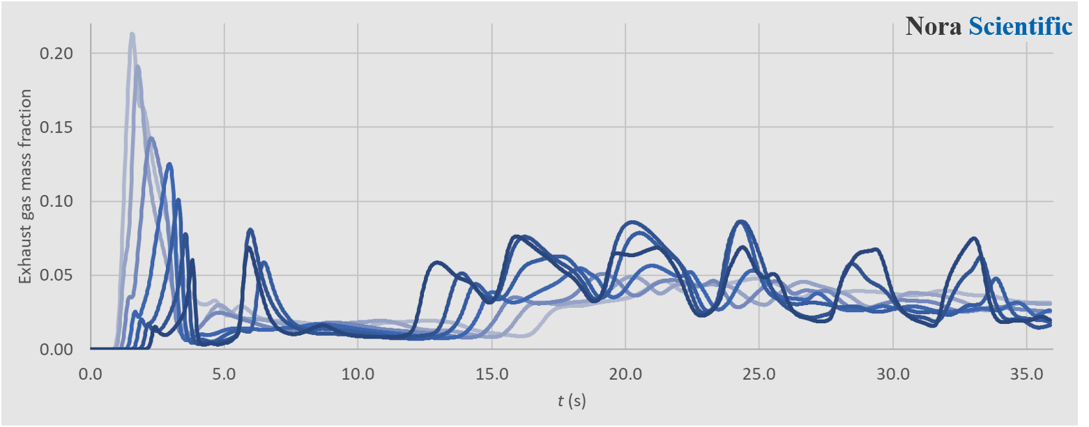
Air Pollution on Cruise Ship Decks
1. Introduction
In January 2019, Business Insider has reported that "the air on cruise ships can be as polluted as the air in Beijing, new study claims" as quoted below.Air pollution on cruise ship decks may be as bad as in cities like Beijing and Santiago, Chile, according to a new study from researchers at Johns Hopkins University.
The study measured pollution levels on the decks of four cruise ships — Carnival Liberty, Carnival Freedom, Holland America MS Amsterdam, and Emerald Princess — in front of and behind the ship's smokestacks.
Pollution behind the smokestacks, including in areas intended for exercises like basketball courts and running tracks, was much worse than in front of the smokestacks, according to the study.
In this tutorial, we construct a model ship funnel by using paint images, and perofrm a flow simulation of exhaust gas from the funnel to understand the mechanism of ship deck pollution.
All the required input files for this test case can be downloaded below.
入力ファイル
The computational time of this case is approximately 20-40 minutes per 1000 time steps with a typical Core i7 PC with the maximum parallelism setting (parallel = 4 in parameter setting).
2. 3D model construction
General rules of constructing 3D boundary conditions using paint images are explained in here. In the present simulation, following five paint images are used to construct the model of a ship funnel. The four colors used in the paint images and parts these colors specify are:
- Wall boundary: outer funnel (decorative funnel cover, non-preset color, purple)
- Inflow boundary: inner funnel (exit of the exhaust gas, preset color, red)
- Wall boundary: deck of the cruise ship (preset color, black)
- Inflow boundary (preset color, green)
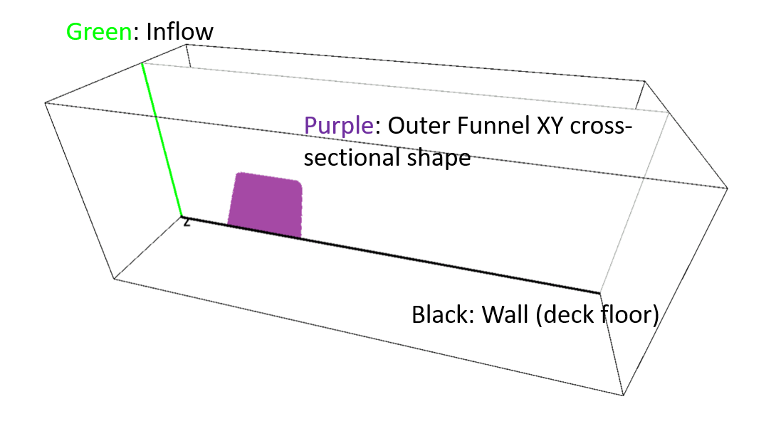
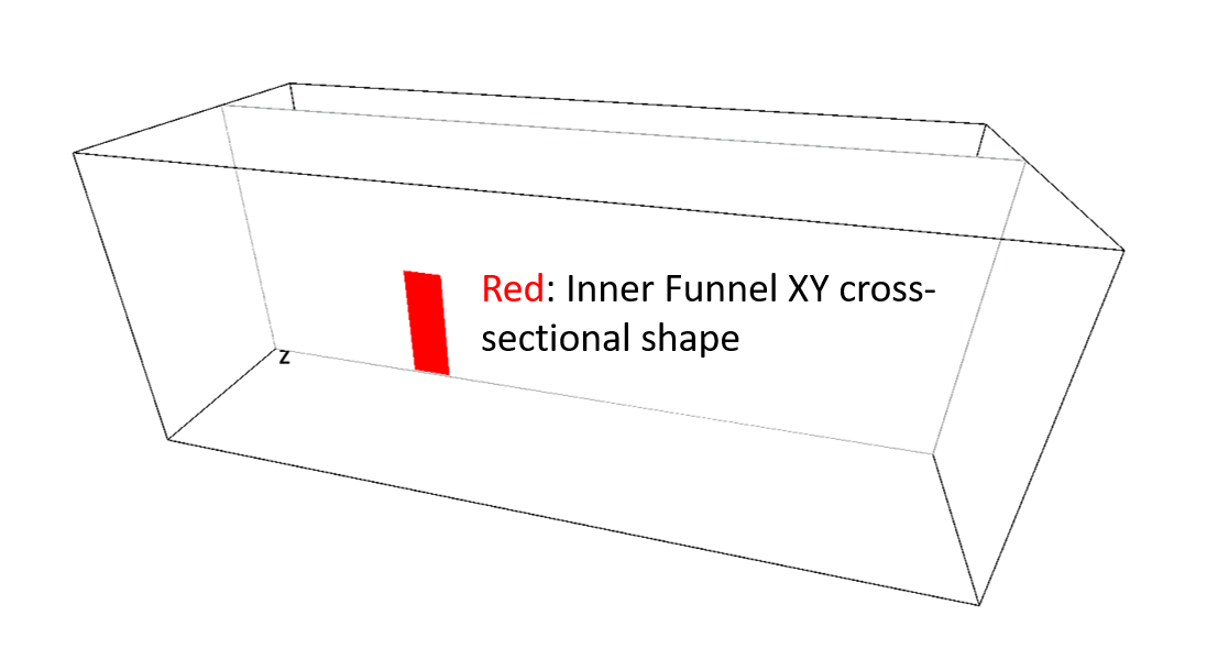
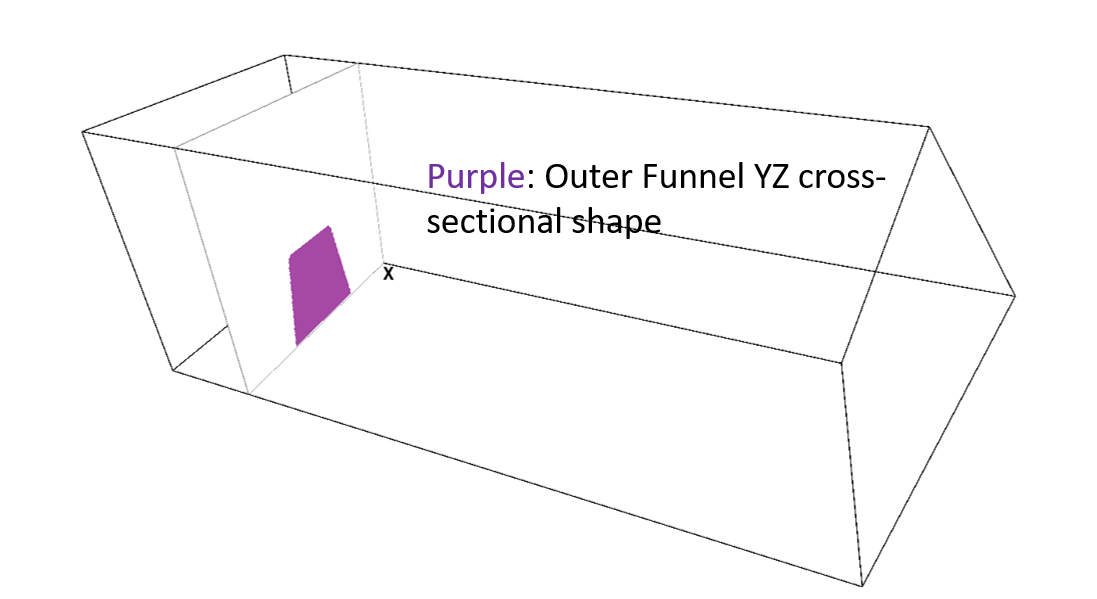
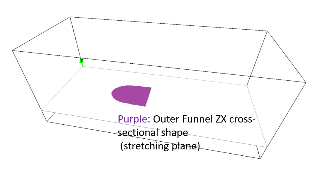
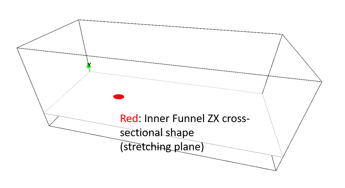
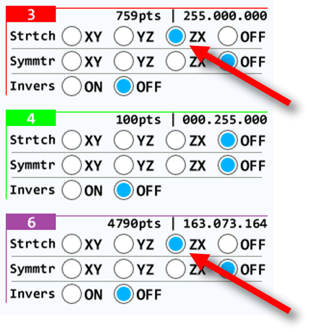
These parts are specified and constructed by using the techniques of (a) Model with a uniform 2D cross-section and (d) Model with a smoothly-changing 2D cross-section (Stretching tool). Here, the outer (purple) and inner (red) funnels are constructed based by using the stretching tool. To do that, select which plane to stretch for these colors by using the ckeckbox (annotated by red arrows) as shown in the right figure.
The paint image pixel sizes can be irrelevant to actual physical domain dimensions. The model dimensions are specified by the parameters, lx, ly and lz. However, it is a good habit to use more or less similar aspect ratio between images and domain dimensions.
3. Numerical parameters
Several important parameters are explained here. Most important parameters are marked by **. More thorough information about parameters can be found here.
- cmode
cmode is taken as 0 for the 0:Fluid simulation mode (constant temperature flows). - lx
The domain length in X-direction is 25m. - ly
The domain length in Y-direction is 10m. - lz
The domain length in Z-direction is 10m. - nx、ny、nz
(nx, ny, nz) = (250, 100, 100) - uinW
Initial x-component fluid velocity is taken as uinW = 10m/s (=19 knots). The other components (vinW, winW) are zero (=default value), so they do not need to be specified. - massfrW**
Initial concentration (mass fraction) in the simulation domain is zero. This is the default value of the parameter, so it does not need to be specified explicitly. - vinR
Velocity (vertical) of the exhaust gas exit from the funnel is taken as vinR = 2.0m/s. The other components (uinR, winR) are zero (=default value), so they do not need to be specified. - massfrR**
The concentration (mass fraction) of the exhaust gas fed from the funnel is 1 (=100%). *exhaust gas concentration: mass fraction of the exhaust gas consisting of the mixture at a given location. - uinG
The x-component velocity from the inflow boundary is taken as uinG = 10m/s (=19 knots). The other components (vinG, winG) are zero (=default value), so they do not need to be specified. Also, the green inflow is used instead of blue. This is because the tracer particles are fed only from the red and blue boundary, and using green inflow as the main inflow boundary is suited to highlight the particle trajectories from the funnel.
4. Performing simulations, post-analysis
Let's start the simulation. You can visualize the flow field during and/or after the simulation (using the analysis mode). However, the present simulation takes a lot of computational time, it would be more suitable to perform detailed visualization after the simulation (the tracer particle visualization can be only perofrmed during the simulation). The below image shows a typical instantanoues exhaust gas concentration field.
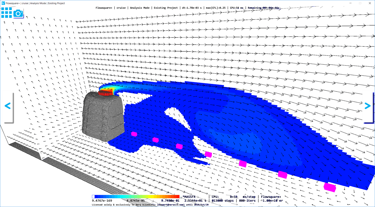
As shown by the tracer particle movements in the below movie, the fluid issued from the funnel periodically rolls towards the deck and towards the upstream. This large flow structure is due to the Kelvin-Helmholtz instabilities that is caused at the interface of fast and slow fluid motions. Because of the large scale vortical motion, the exhaust gas exit from the funnel actually pass through the deck towards the leeward of the funnel.
This is a good example of how CFD can be used to reveal the mechanism of the phenomena observed in measurement such as the above report.
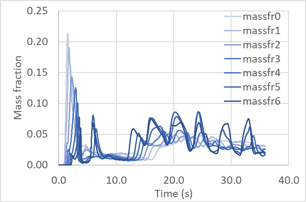
Also, the exhaust gas concentration evolution over time measured at seven probes located as in the above movie is blow. You can see how to use probe tools in Flowsquare+ here.
In this simulation, the temperature difference between surrounding and exhaust gas and buoyancy are not conisdered. Flowsquare+ can also include these effects and you can see such an example simulation here.