The Easiest Computational Fluid Dynamics Software
 JP
JP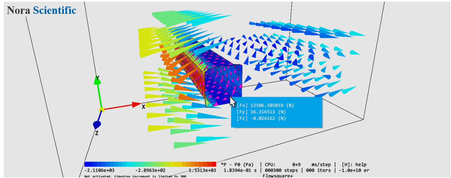
Getting Familiar with the Interface
Display items in the simulation windows and various tools for understanding of the flow field are explained.
- Window size, language, and graphic settings
- Parameter editor
- 2. i. Descriptions of the items in the Parameter editor
- 2. ii. Direct access to the boundary configuration bitmap images
- Boundary configuration image loader
- Boundary confirmation/CAD model loader
- Interface during simulation and analysis
- 3D visualization mouse operation
- Pointwise data inspection
- Tool pane
- Cross-section position
- Placing probes
- Hydrodynamic force measurement
- Tracer particle
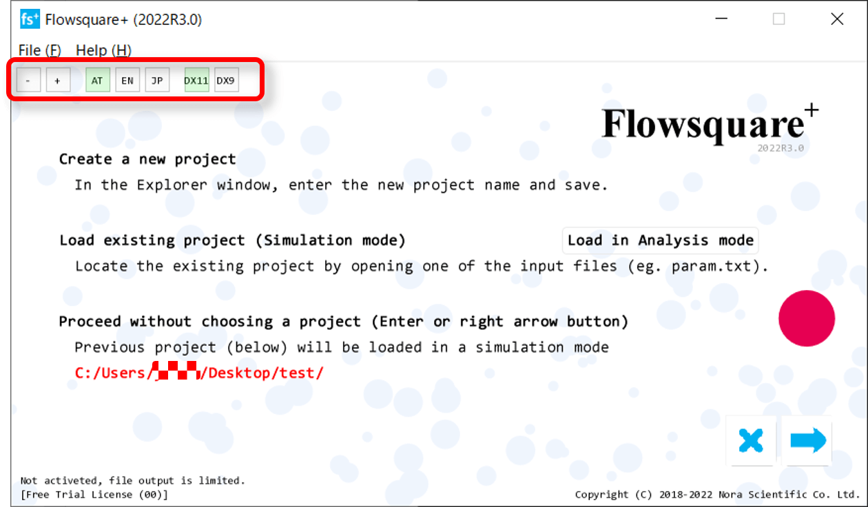
1. Window size, language and graphic settings
2022R1.0 or laterSoftware's window size, language and graphic settings can be set as follows.
Window size
- [-] Smaller window size.
- [+] Larger window size.
*On a par with general Windows applications, you can also change the window size in Flowsquare+, by dragging the outer edge of the window.
Language
- [AT] Software's language as the same as OS's language setting
- [EN] Software's language as English
- [JP] Software's language as Japanese
Graphic
- [DX11] Graphic by DirectX 11 (default).
- [DX9] Graphic by DirectX 9.
*For few graphic cards and driver versions, 2022R2.0 or earlier versions consumes significant amount of RAM, during graphic processes in Flowsquare+ using DirectX 11. This is due to the implementation of the driver software. To avoid this issue, the user can choose DirectX 9 instead of DirectX 11 in 2022R3.0.
2. Parameter editor
The parameter editor loads param.txt and shows many informations, but the general rule is this: each line contains all the information of a parameter, such as parameter name, parameter value (in form of a number or a radio button), parameter description. A part of parameter description is displayed on the right part of the window, but by hovering a mouse pointer on the row of your interested parameter, the entire parameter description will be displayed.
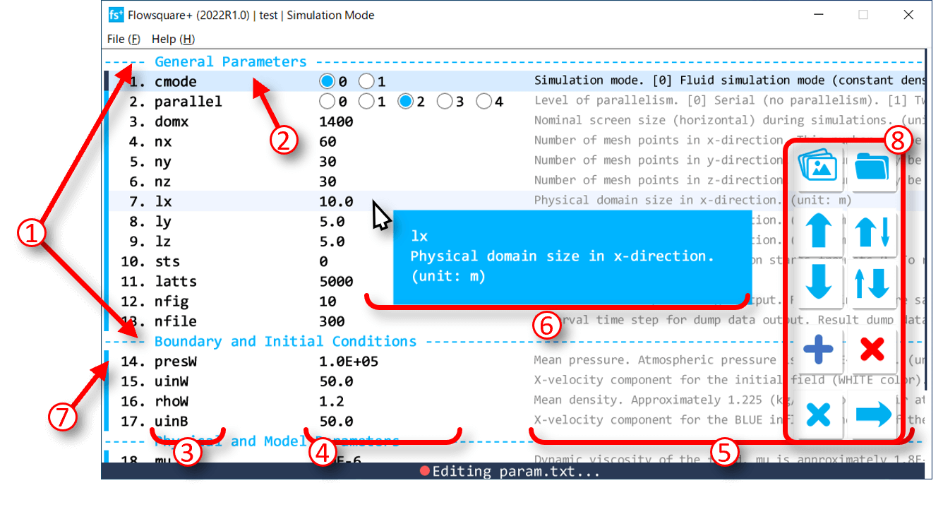
i. Descriptions of the items in the Parameter editor
- Divider between parameter rows
For better readability, dividers can be placed. All dividers begin with "-" (hyphen). - Active parameter row
You can select an active parameter row with click, /
/ buttons, and arrow keys.
 - Parameter name
- Parameter value
Parameter value can be set by a text input or a radio button. - Parameter description (partial)
- Parameter description (full)
Full description of a parameter is shown with mouse over. - Parameter validity flag
- ■: Parameter name is valid, and the parameter is effective
- □:Parameter name is valid, but the parameter is ineffective, due to the values of other parameters
- ■:Parameter name is invalid
- Parameter editor buttons
 To open the list of bitmap images for boundary configuration [2022R1.0 or later]
 To open the current project folder in Explorer [2022R1.0 or later]
- To move up.
- To move down.
 Swap the parameter row and move up.
 Swap the parameter row and move down.
 Add a new parameter row or a divider row. To add parameter, type a parameter name and press the OK button. To add a divider, type any string you like which begins with "-" (hyphen).
 Remove a parameter row.
 To cancel.
 To proceed.
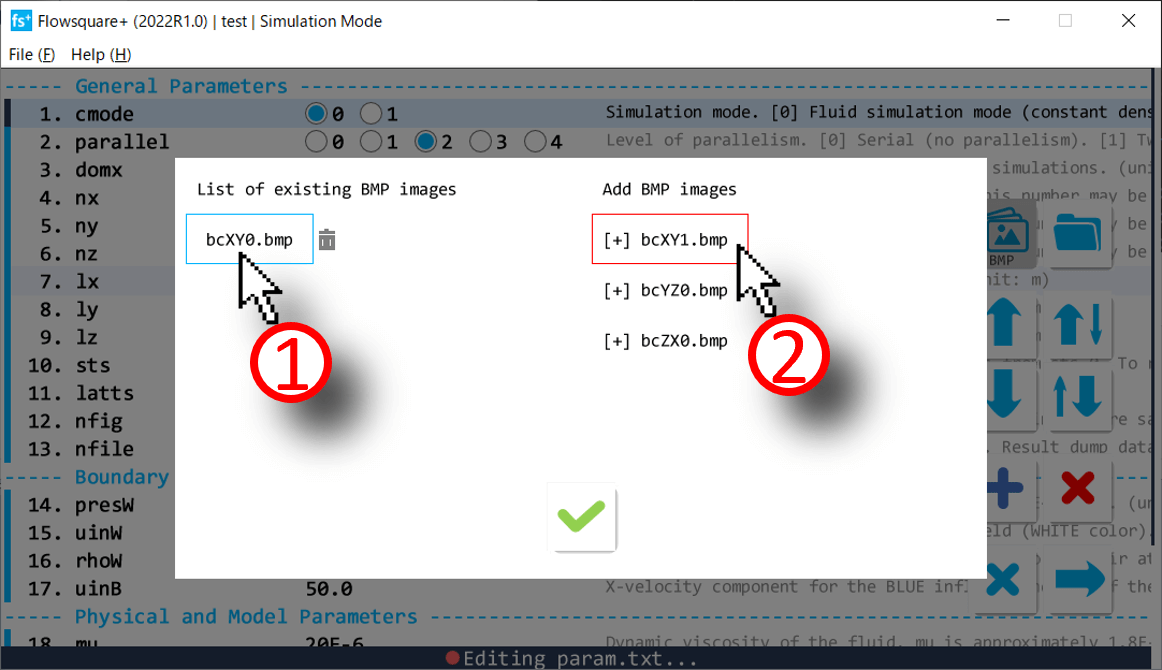
ii. Direct access to the boundary configuration bitmap images
[2022R1.0 or later]Using , you can view the list of boundary-configration bitmap images in the present project (figure below). From this list, you can open an bitmap image with the Paint software (click (1) in the below figure) or create a new bitmap image (click (2) in the below figure).
Note that while eiditing a bitmap image directly opened from the list in the below figure, Flowsquare+ does not accept any operation. You need to (save and) close the Paint before you can use Flowsquare+. Also, you can create up to 10 bitmap images for each direction. For example, for XY images, you can create bcXY0-bcXY9.
By clicking a bin icon next to the bitmap image name in the list, you can delete the image from the project.
3. Boundary configuration image loader
Boundary configuration images (bcXY0.bmp, etc..) are loaded and displayed with physical dimensions aspect, and the computational mesh specified in param.txt is overlaid on each image. There are few configuration options on the right hand side of the window for each colour including both preset and non-preset colours.
Boundary conditions defined by preset and non-preset colors are constructed in the color order in the list shown in the below figure (constructed from top to bottom colors in the list). This color order can be modified by drag & drop as shown in the below figure. If more than one boundary conditions defined by different colors conflict, the boundary condition constructed later is priotized and overwrites the other.
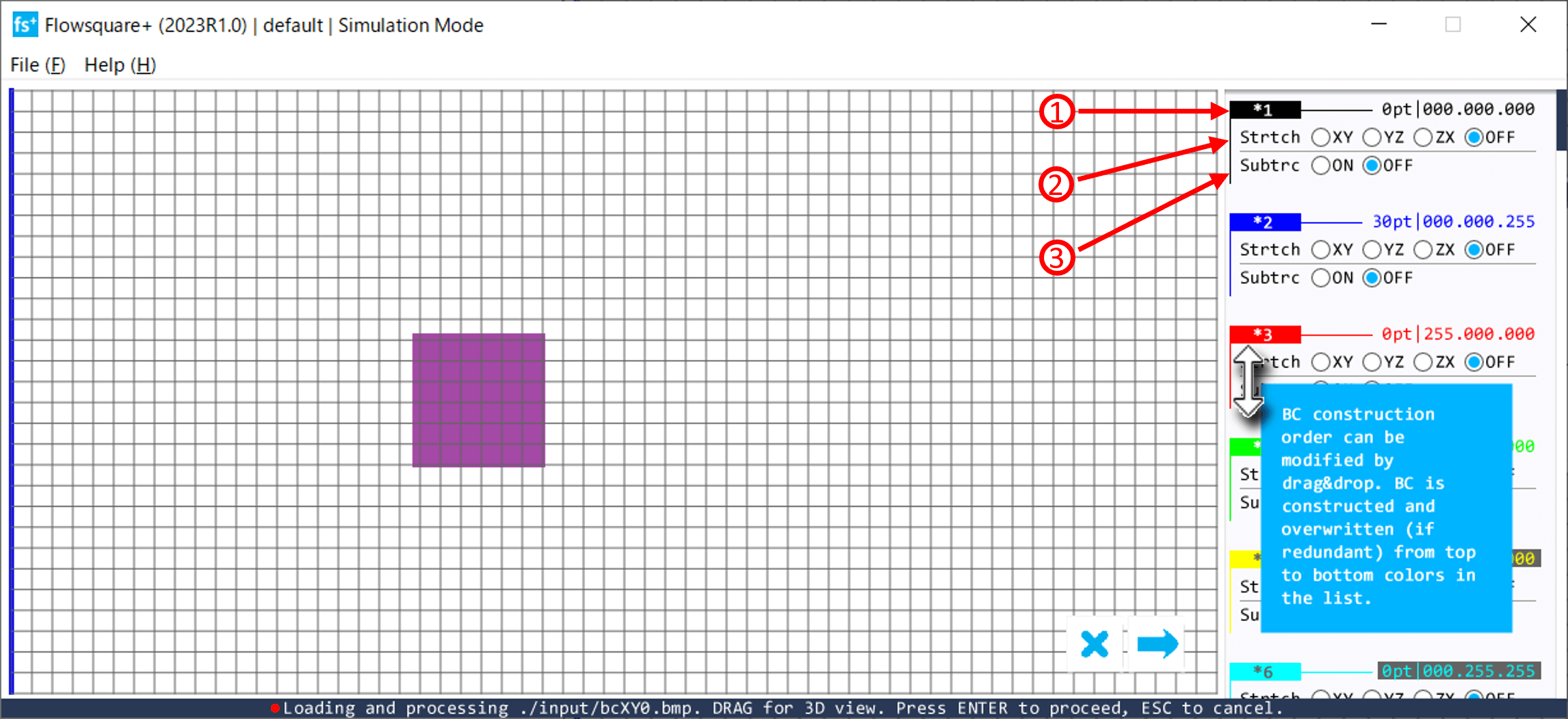
Descriptions of the numbered items in the above figure.
- Colour information
Information of each colour used in the boundary configuration images. Preset colours (denoted by * mark on the left of color index) are always shown whether used or not. - Strtch
Radio buttons to specify "Stretching" operation plane for each colour. A shape of the corresponding colour in the specified plane will be stretched. - Subtrc
Radio buttons to specify subtraction (Subtrc) of the target object from a model(s) consisting of other colors. Here, the model construction order of each color needs to be appropriately set. The model color to subtract must be placed after the model color to be subtracted (drag-and-drop operation in the color list to change the order).
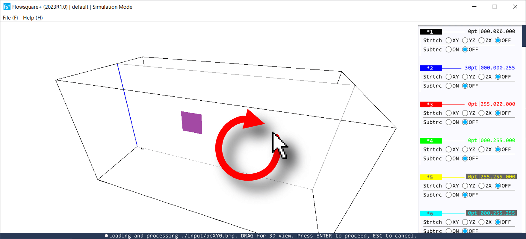
Checking the placement direction of loaded image
With a left-drag mouse operation within the domain area, the direction of the displayed image can be viewed in the 3D simulation domain.
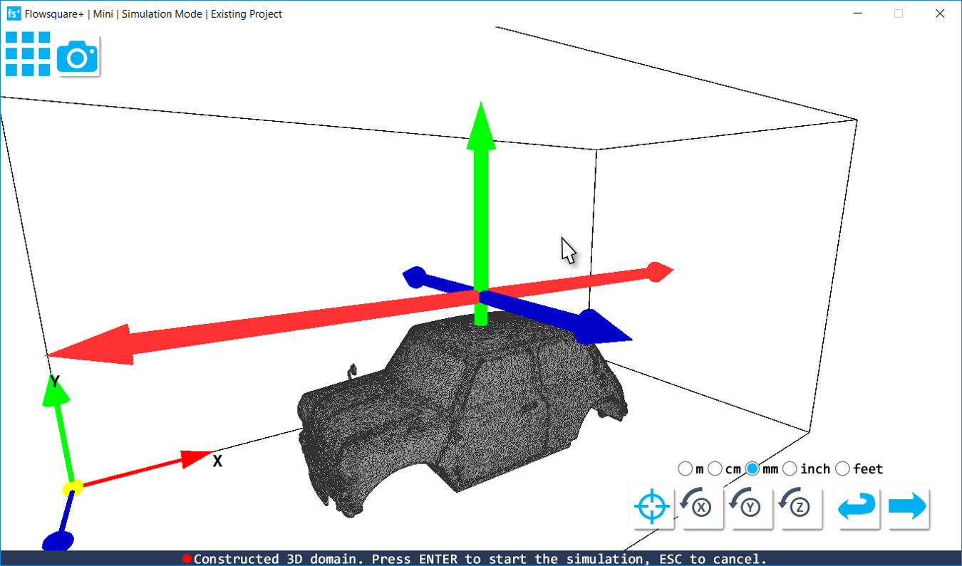
4. Boundary confirmation/CAD model loader
After all the boundary configuration images are loaded in Sec. 2, a CAD model (bc.stl) is loaded if necessary.
The CAD model is then constructed and displayed based on the default parameters and/or settings in param.txt. You may further adjust the CAD model, such as position, direction, used unit, by using the below interface.
![Shifting the STL model position with [SHIFT] + [Mouse Drag].](images/tutorial/315_STL_shift.png)
Descriptions of mouse operation
Follwoing mouse operations can be used to adjust visualization of the 3D domain.
- Left drag: to rotate the simulation domain
- Right drag: to move the simulation domain
- Scroll: zoom-in/-out the simulation domain
Procedure to change the CAD model position in the domain
- Overlay the mouse cursor on one of large arrows, along which you want to move the CAD model, displayed on the center of the domain.
- Once the arrow is displayed in the magenta color, press SHIFT key while left dragging to the direction you want to move the CAD model.
Descriptions of the interface of the CAD model loader
 Move the CAD model to the center position of the simulation domain.
 To rotate the CAD model by 90 degrees around X-axis.
 To rotate the CAD model by 90 degrees around Y-axis.
 To rotate the CAD model by 90 degrees around Z-axis.
- Radio buttons: To change unit in the STL file (m, cm, mm, inch, feet)
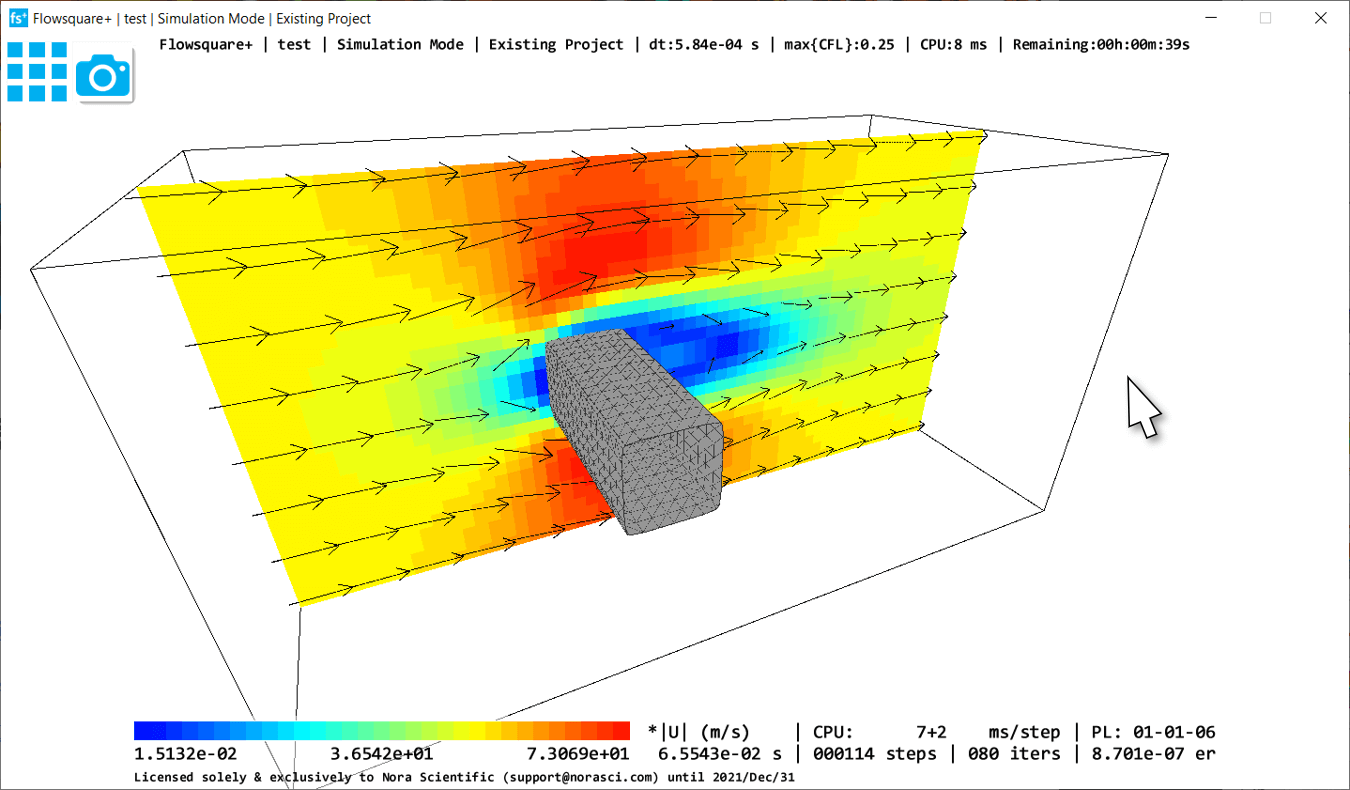
5. Interface during simulation and analysis
There are many information shown during the simulation, and they are explained below.
Descriptions of mouse operation
Follwoing mouse operations can be used to adjust visualization of the 3D domain.
- Left drag: to rotate the simulation domain
- Right drag: to move the simulation domain
- Scroll: zoom-in/-out the simulation domain
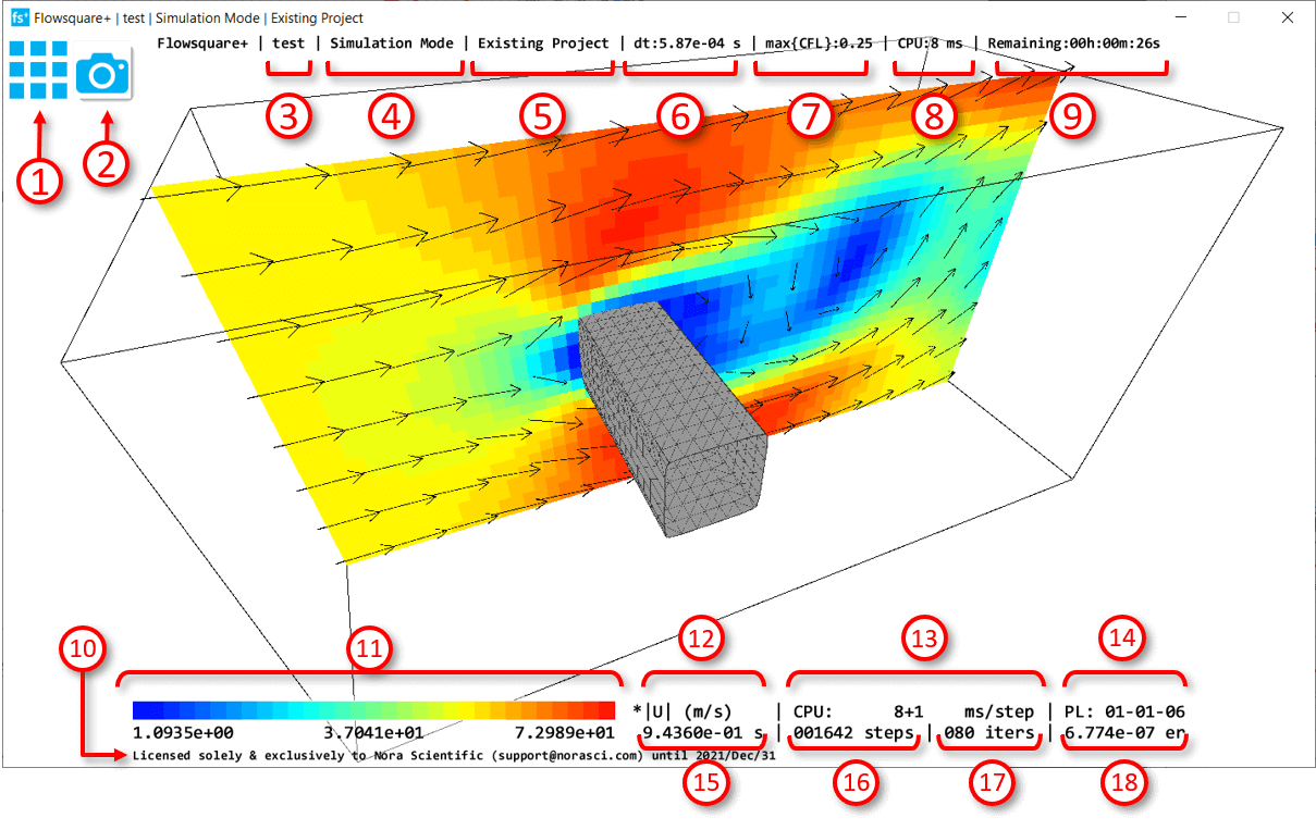
Descriptions of the numbered items in the above figure.
- Tool pane button.
(*This button is shown when the window is active and the mouse cursor is located inside the window). - Snapshot (screen capture) button.
- Project name.
- Execution mode
Simulation Mode or Analysis Mode). - Project newness
New Project or Existing Project. - Time step size (Δt).
- Maximum CFL number.
- Averaged computational time per time step, averaged over the latest 20 time steps (in ms).
- Estimated remaining time based on the averaged computational time.
- License information.
- Colorbar of the displayed quantity, and its minimum, middle and maximum values.
Click the displayed color bar during the simulation to change the colormap. There are five different colormaps. 1. Rainbow
 2. Nishiki
 3. Hot
 4. Grey scale
 5. Grey scale (inverted)
- Name of the displayed quantity.
- RHO (kg/m^3): Fluid density (kg/m^3), only for thermo-fluid simulation; cmode = 1.
- U (m/s): Velocity component in X-direction (m/s).
- V (m/s): Velocity component in Y-direction (m/s).
- W (m/s): Velocity component in Z-direction (m/s).
- |U| (m/s): Magnitude of velcotiy (m/s).
- T (K): Temperature (K), only for thermo-fluid simulation; cmode = 1.
- MASSFR: (Mass) fraction of scalar (species/pollutant/etc..).
- P - P0 (Pa): Pressure (minus initial mean pressure; presW).
- Computational time of most recent time step (in ms)
Computational time regarding solving transport equations + computational time regarding visualization. - Number of parallelism used for current parallel computation
The three numbers correspond to npx, npy, npz, which are number of threads used for x, y, and z-directions. The total number of threads is npx*npy*npz. - Physical time of current time step
Beginning of the simulation corresponds to t=0 (s), and the physical time is calculated by accummulating Δt over time steps. - Current time step
- Number of iterative computation until convergence
- Residual error (relative to the initial value)
Buttons displayed during analysis mode
 To load previous dump data saved for a smaller timestep.
 To load next dump data saved for a larger timestep.
6. 3D visualization mouse operation
In the boundary confirmation display, CAD model loader, simulation and analysis display, several mouse operation is available to adjust 3D visualization.
- Left drag
To change the camera angle. - Right drag
To change the camera focul point. - Scroll
To change the distance between camera focul point and camera position.
7. Pointwise data inspection
Flowsquare+ can display physical quantity information at any point in a 2D simulation domain, or at any point on an arbitrary 2D cross-section plane displayed in a 3D simulation domain. To display the information, move the mouse cursor to the coordinate you want to inspect and press the SHIFT key. The coordinate position and the value of the currently displayed physical quantity will appear next to the mouse cursor.
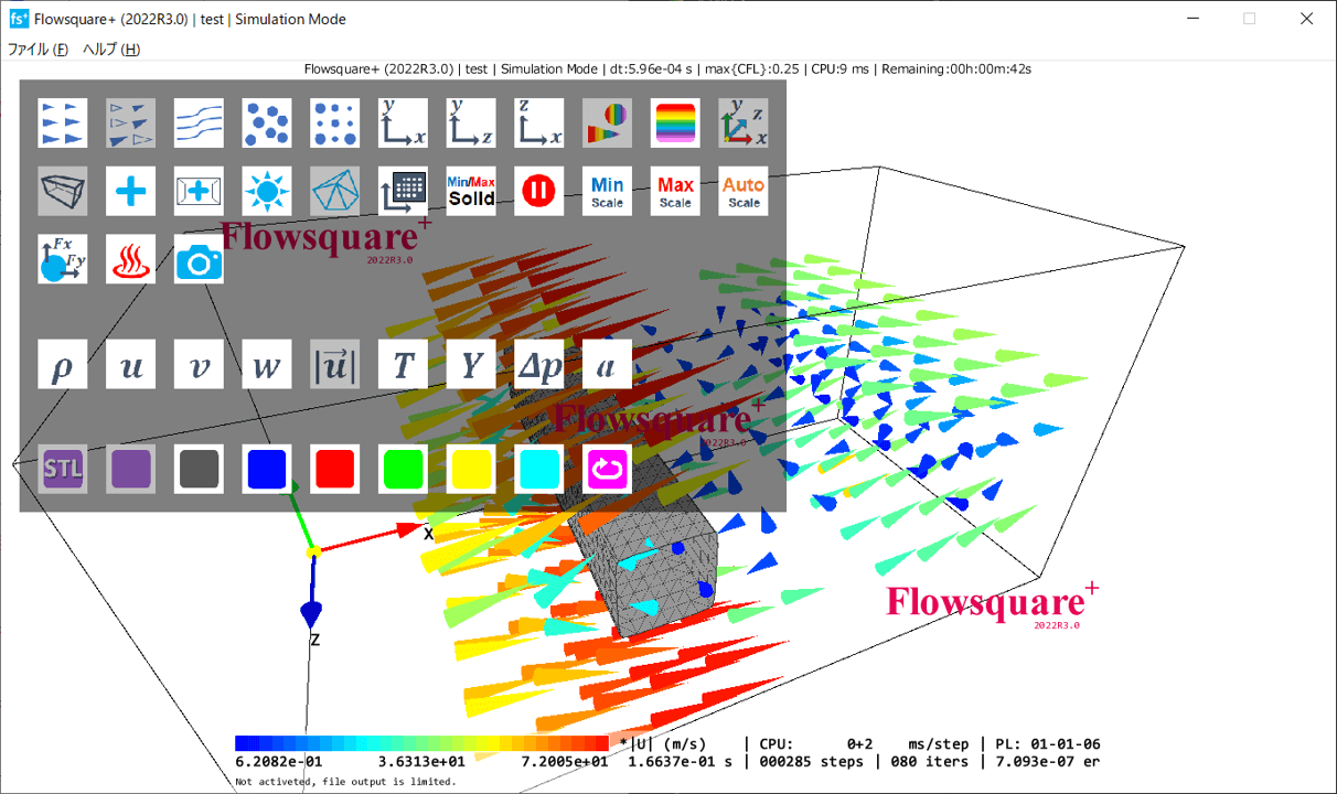
8. Tool pane
Hover the mouse pointer on the tool pane icon  , and the tool pane will appears. There are many visualization tools are available, and you can choose these tool during a simulation and analysis phases.
Note that Flowsquare+ detects these interface operations at the switchover of each time step, and the changes will reflect in the next time step. Therefore, if the simulation is relatively computationally demanding and slow, you may see a delay in these processes.
 Velocity vector
 *Uncorrelated velocity vector (displays velocity vectors that are uncorrelated with blue inflow velocity)
 Streamline
 Tracer particle (demo)
 *Contour particle
 *XY cross-section. While pressing SHIFT key, mouse scroll on the cross-section to move it.
 *YZ cross-section. While pressing SHIFT key, mouse scroll on the cross-section to move it.
 *ZX cross-section. While pressing SHIFT key, mouse scroll on the cross-section to move it.
 Colouring visualization object based on the current physical quantity
 *Colouring boundary conditions based on the current physical quantity
 *To display CAD (STL) specified boundary conditions
 To display non-preset-colour specified boundary conditions
 To display black-colour specified boundary conditions
 To display blue-colour specified boundary conditions
 To display red-colour specified boundary conditions
 To display green-colour specified boundary conditions
 To display yellow-colour specified boundary conditions [2021R1.0 or later]
 To display cyan-colour specified boundary conditions [2021R1.0 or later]
 To display magenta-colour specified boundary conditions [2022R1.0 or later]
 *Orientation axes
 *Domain outline
 *Camera target
 *Reset camera
 *3D lighting
 *Polygon frame
 *Ghost/solid regions. Computational mesh points specified as wall or inflow boudaries are highlighted by points on the XY, YZ, and/or ZX planes.
 To include the ghost/solid regions in min/max values
 Pause the simulation
 Manually setting a minimum value in the color scale [2019R3 or later]
 Manually setting a maximum value in the color scale [2019R3 or later]
 Automatically setting minimum and maximum values in the color scale [2019R3 or later]
 Density
 U
U
 V
V
 *W
*W
 Magnitude of velocity
 Temperature
 Mass fraction
 Pressure
 Age variable [2021R1.0 or later]
 Hydrodynamic force measurement (details)
 Wall heat flux measurement. *The heat flux is computed as \(\Phi_{wall}=k|\partial \tilde{T} / \partial x|\), and no SGS contribution is considered (a model to be included in future update). The variable notations are the same as description of solver page.[2021R1.0 or later]
 Snapshot (screenshot)
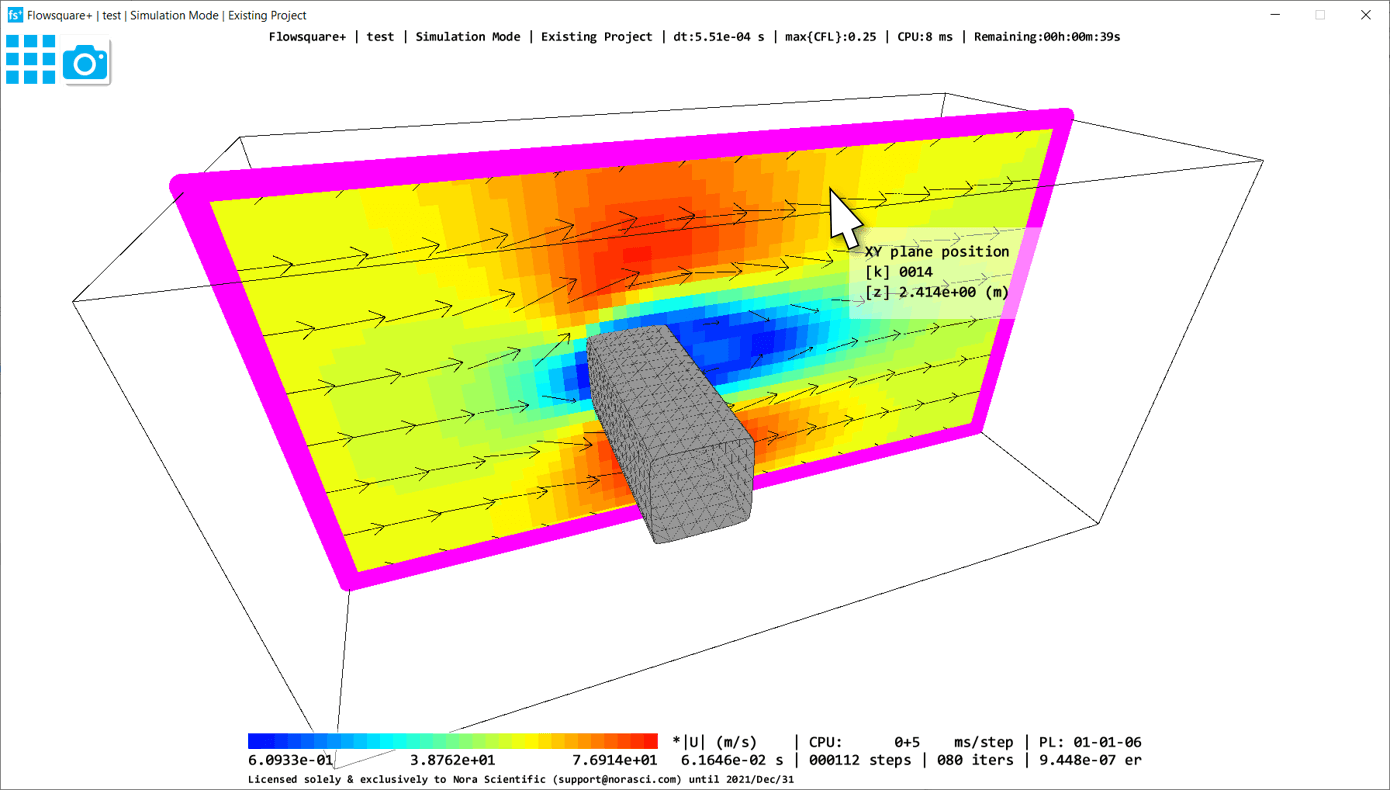
9. Cross-section position
In the simulation and analysis modes, you can dislplay XY, YZ and ZX cross-section plane(s) in your 3D simulation domain by using , and in the tool pane.
To change the position of these cross-section planes,
- Move the mouse cursor on the cross-section you want to move, and press SHIFT key. Then the plane will be highlighted and its position is displayed as in the image below (eg. XY plane position).
- While the plane is highlighted, rotate the mouse scroll wheel.
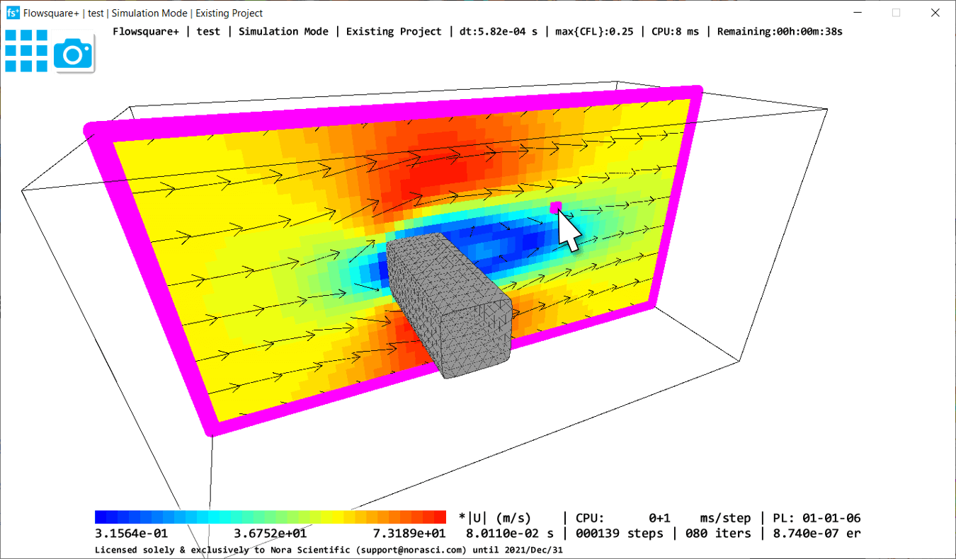
10. Placing probes
In Flowsquare+, you can place measuring probes. The probes can measure and store temporal evolution of physical quantities along with the time, and the results are saved in the ./dump directory in a project folder. Probe measurement will be resumed automatically, when you restart the simulation.
Below explains how to use the probes, using the test case we've already used.
i. Display XY, YZ, or ZX cross-section planes
Referring "Flowsquare+ for Beginners", perform a simulation with the test case input files. Once the simulation has started, display XY, YZ, or ZX cross-section plane using , , or button in the tool pane.
Move the displayed cross-section plane so that the position of the probe you want to set belongs to the plane (you can move the plane by mouse scrolling on it while pressing SHIFT key).
ii. Click on the cross-section plane while pressing SHIFT key
Move the mouse cursor to the position where you want to place a probe on the cross-section plane, and click while pressing SHIFT key. A probe will be set on the location on the cross-section plane you clicked on, and displayed as a megenta cube (■) in the simulation domain.
iii. Placing multiple probes, discarding probes
By repeating above procedures 1 and 2, you can place maximum of 10 probes in the simulation domain. Also, you can erase probes by right clicking while pressing SHIFT key. Probes are erasec from newer to older order.
iv. Probe measurement result file
Probes are allotted a number from 0 (first to set) to 10 (last to set), and measured results are stored in the ./dump directory in the project folder. Their file name contains the number allotted for each probe. Each probe contains following information at each measurement time (initially set as once in every ten timesteps):
- ts, time step
- time(s), time
- x, y, z(m), probe location
- rho(kg/m^3), density
- U(m/s), X-direction velocity component
- V(m/s), Y-direction velocity component
- W(m/s), Z-direction velocity component
- T(K), temperature
- massfr, mass fraction
- dP(Pa), pressure (P-presW)
The probe file (e.g. probe_000_ascii.dat) can be opend by any spreadsheet software such as Microsoft Excel, and you can generate temporal evolution plots.
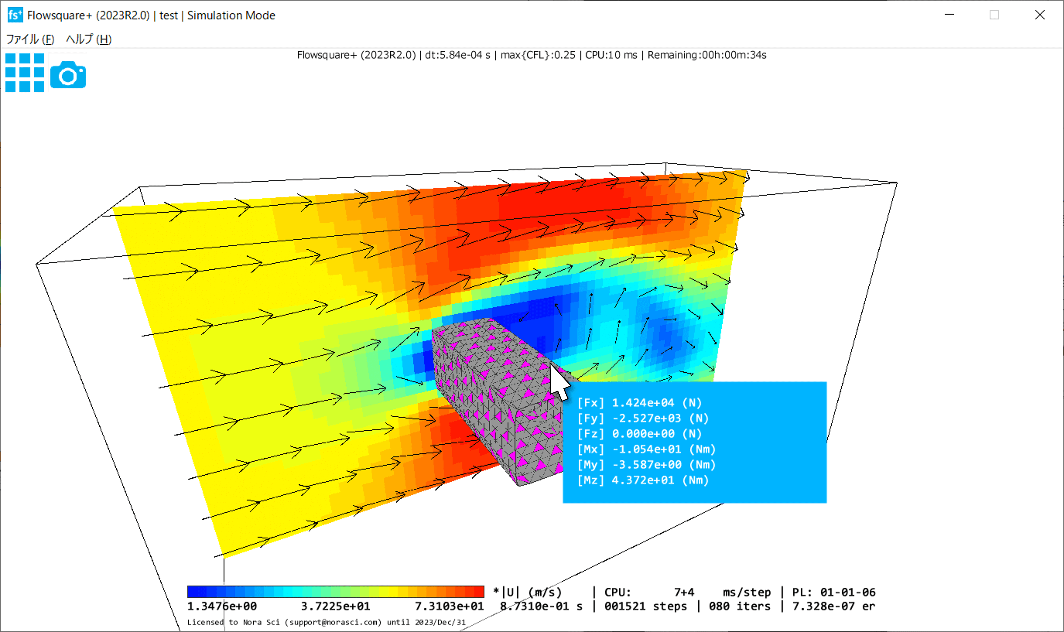
11. Hydrodynamic force measurement
You can calculate the hydrodynamic forces (drag, lift, downforce, moments, etc...) acting on solid objects (wall boundaries) in the simulation domain, and save the time history of these forces. Press button in the tool pane to activate the environment for hydrodynamic force computation. Then, move the mouse pointer onto the object of interest in the simulation domain. The object is highlighted by the magenta color ■, and the component of the fluid force and moment in each direction will be displayed as in the below image (e.g. "Fx" is the force in x-direction, and "Mx" is the moment in x-direction).
*Here, the reference point of the moment calculation is defined by the parameter "refMoment". By default, "refMoment" is set such that the reference point is the center of gravity of the object assuming constant density.
Note that the unit length (1m) of the out-of-plane dimension is assumed for the computation of the hydrodynamic force for 2D simulations.
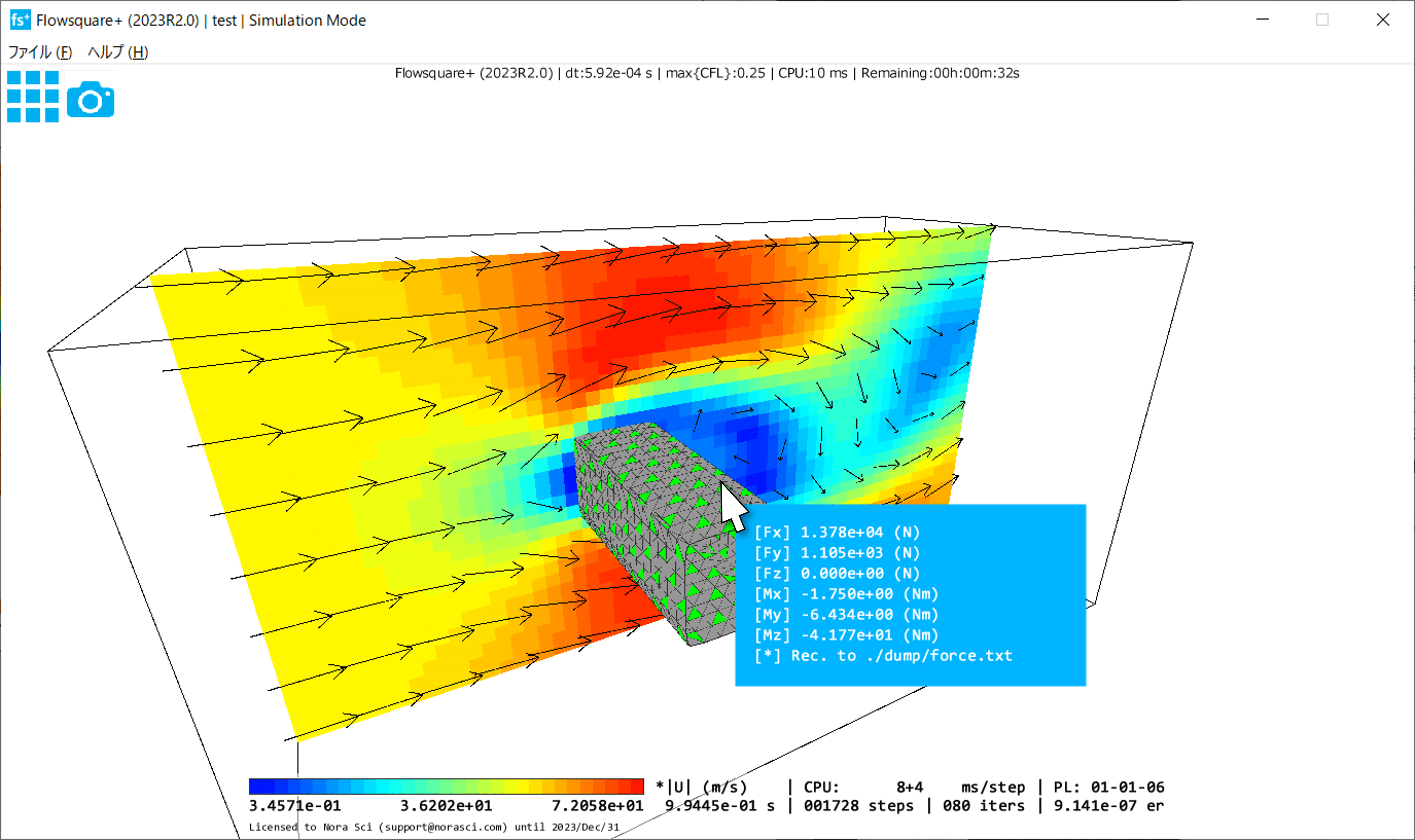
While the object of interest is highlighted by the magenta color ■, left-click to start recording the time history of the force. Once the recording is started, the object will be highlighted by the green color ■, and the data is saved as force.txt in the dump directory in the project directory. force.txt can be opened by a text editor or Excel, and all boundaries, physical quantities and units are appropriately labelled so they are self-explanatory.
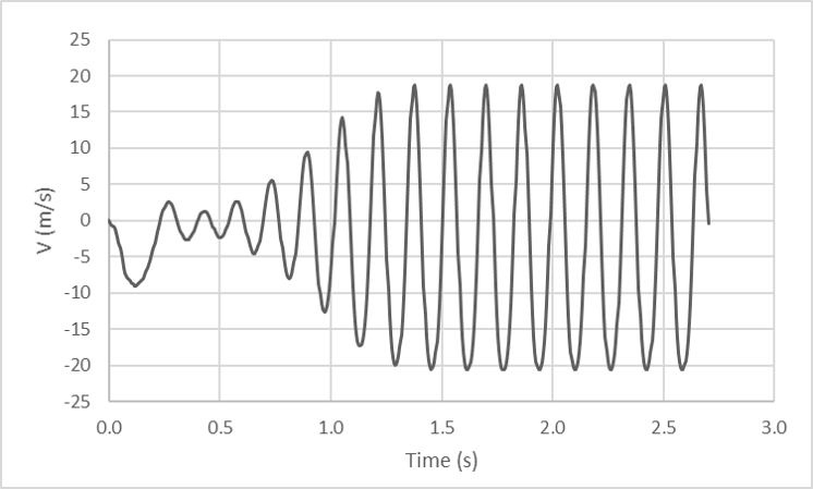
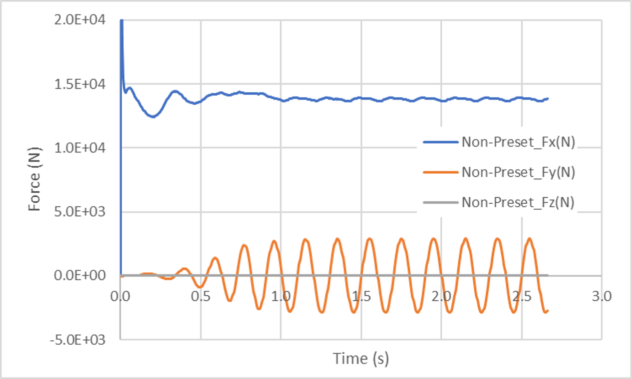
The below image shows an exmaple plot of hydrodynamic forces recorded for an object constructed by non-preset colors (Non-Preset), using force.txt.
Version information related to the hydrodynamic force measurement
- Hydrodynamic force for 3D simulation [2019R1.0 or later]
- Hydrodynamic force for 3D simulation [2020R2.0 or later]
- Recording of measured forces [2020R2.0 or later]
- Computing and recording of fluid moment [2023R2.0 or later]
12. Tracer particle
Plese see here for details.