The Easiest Computational Fluid Dynamics Software
 JP
JP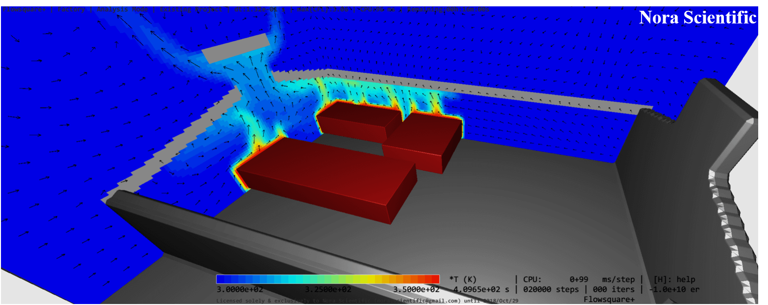
Tips to Improve Your Simulations
General aspects of computational fluid dynamics (CFD) are explained. For more detailed mathematical information on the simulation solver used in Flowsquare+, see this page.
1. Introduction
Using Flowsquare+ with modified input files available for the example cases allows everyone to perform their own simulation straightforwardly. The visualization tool included in the software can render the simulation solution in a colourful manner so that the solution looks convincing.
This page explains how to improve flow simulations, intended for those who perform flow simulations, not only for its own sake, but to use the solution to obtain some insights or for optimization.
More basic aspects of computational fluid dynamics are described in "Basics of CFD". Also, more detailed description of mathematical aspects can be found in "Flowsquare+ Solver".
2. Spatial resolution
Spatial resolution is one of parameters that directly influence solution accuracy and computational cost (computational time). Generally, to accurately simulate entire fluid phenomena, one needs to use high-accuracy numerical scheme with a mesh size, \(\Delta x, \Delta y, \Delta z\), as small as the Kolmogorov length scale, which are considered to be the smallest scale in turbulence. Such a simulation is called direct numerical simulation (DNS) and perofrmin DNS requires a supercomputer due to its large number of mesh points and numerical schemes.
In Flowsquare+, turbulence models (SGS models) are implemented to capture the effect of fluid motion smaller than used mesh size, to reduce computational cost while capturing inherent unsteadiness of fluid flows. Thus, Flowsquare+ can predict flow fields accurately (to the limit of the model accuracy) with much less number of mesh points than DNS.
Contrary, the topology of physical boundary (e.g. walls) smaller than mesh size cannot be captured by any turbulence models. Thus, the user choose how many mesh points to use carefully, by considering the shape of physical boundary and model capability.
That being said, the number of mesh points to be used in CFD on general PC/laptops is typically constrained by the resources (RAM, CPU time). Thus, it would be practically reasonable that the user first optimizes the object shape and the simulation domain, and then uses the largest number of mesh points feasible in their environments.
In Flowsquare+, the mesh specified in the parameter editor is superimposed on the "boundary configuration image loader" display as shwon below, to help the user optimize their mesh points respect to the shape of the physical boundary condition. If the shape of the boundary is not appropriately resolved, it is advisable to adjust the boundary and/or the number of mesh points.
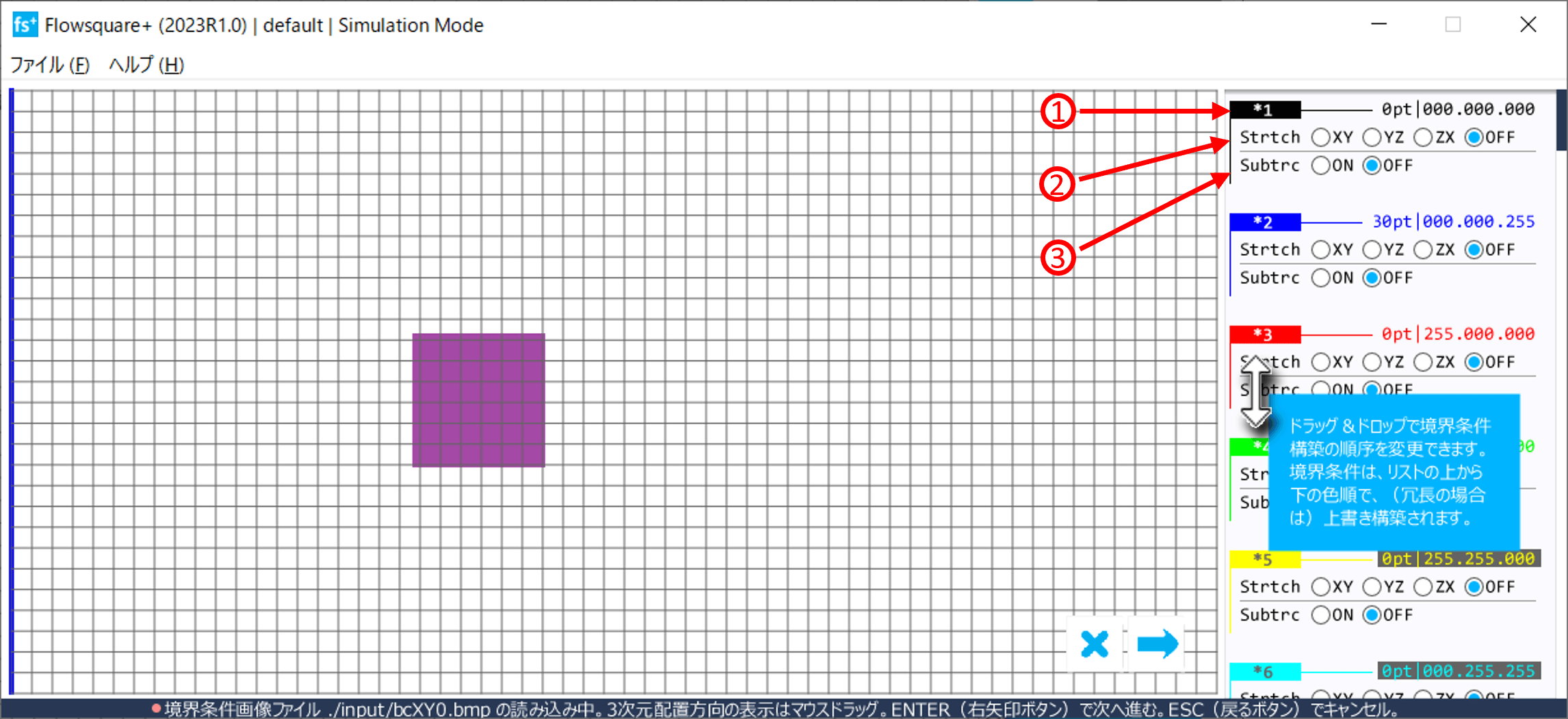
3. Simulation duration
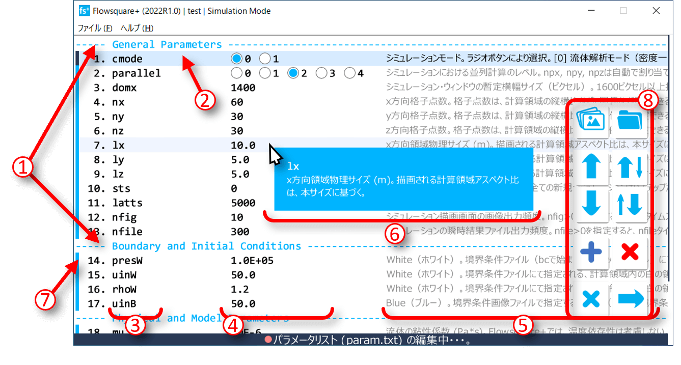
For a constant time step size \(\Delta t\), the physical time \(t\) can be calculated simply by \(t=TS\times\Delta t\), where \(TS\) is the time step. Flowsquare+ dynamically adjusts \(\Delta t\) during the simulation, and the user check the physical time on the Simulation display, or in the output files in the ./dump/ directory.
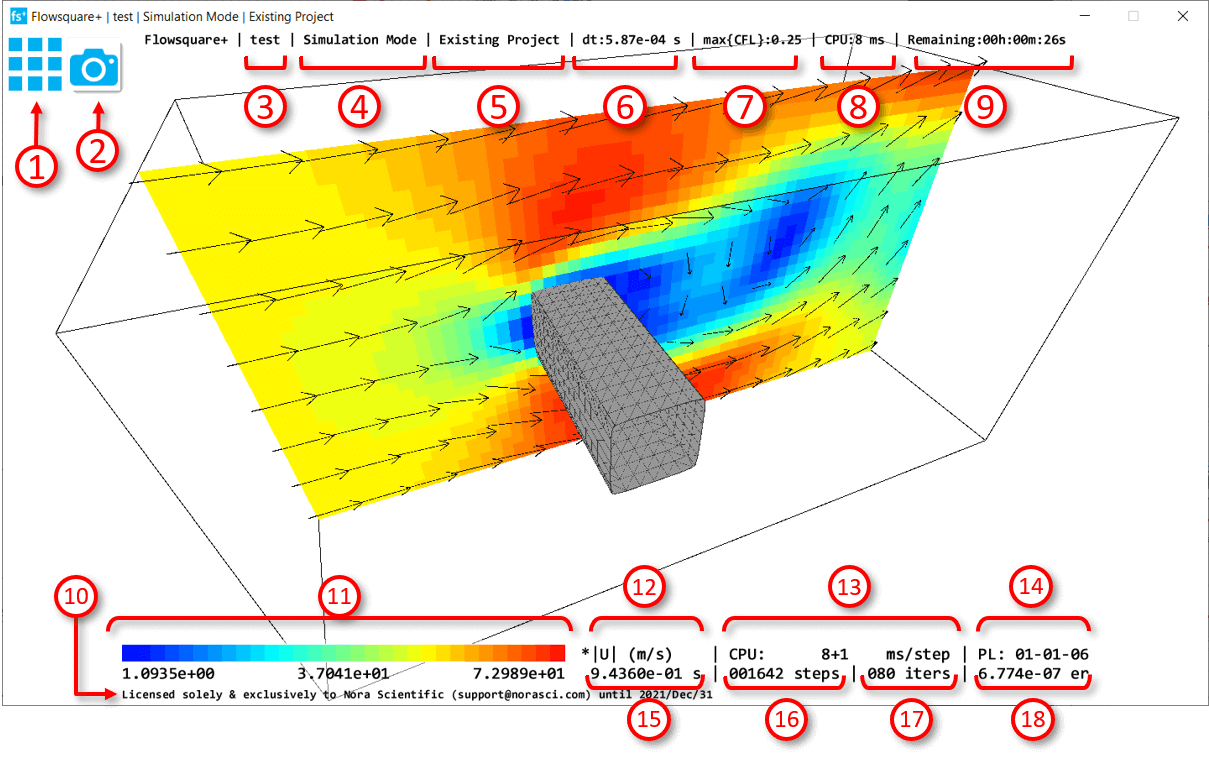
Flowsquare+ initializes the simulation domain with constant physical quantities such as uinW, vinW, winW, rhoW, tempW and/or massfrW (so called impulse start). In many simulations, the solution field is influenced by the initial field. Thus, unless the simulation is performed to see the initial transient of the flow, it needs to be continued long enough so that the initialization effect leaves the simulation domain.
The question here is how long is "long enough"? Here are two easy ways to assess this.
- The easiest way is to estimate the time scale of the flow in the simulation domain, \(\tau\), by \(\tau = L/U\), where \(L\) is the representative length of the simulation domain and \(U\) is the representative velocity in the domain. Usually, a simulation should be continued for about 5 to 10 times of \(\tau\) to minimize the initialization effect on the solution.
- A more rigorous way would be to utilize the probe measurement available in Flowsquare+. As shown below, the velocity variation measured at a probe located in a simulation domein shows quasi-steady state after \(t=1.5 (\rm{s})\). Thus, in this case, the simulation should be continued more than \(t=1.5 (\rm{s})\). Without using probes, the user may assess this by looking at the solution images generated once in every nfig timesteps specified in the parameter.
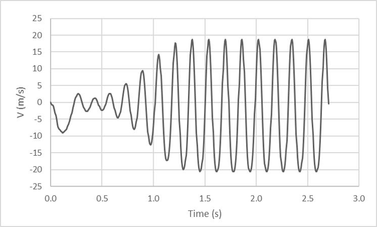
Velocity variation measured at a probe.
4. Choice of simulation domain
If the computational boundaries in your simulation coincide with open boundaries, the size of the simulation domain should be chosen carefully. If the distance between physical boundary (object placed in the domain) is too close to one of the open boundaries, the simulation solution will be unphysically influenced by the computational boundaries. It is generally hard to assess how far the object should be away from the outflow, but this may be approximately the length of the object or more (for some high speed flow condition, this may be 10 times or more of the object length).
5. Residual error and iterative calculation
peps and loopmax are the parameters and are the residual error tolerance and maximum number of iteration calculation. A smaller peps and larger loopmax generally achieves higher accuracy of simulation, but increases computational cost. A larger peps and smaller loopmax increases the computational speed, but lowers the simulation accuracy, and sometimes even leads to divergence of simulation. For most cases, default values works fine, but depending on the simulation environment, these values should be adjusted.