The Easiest Computational Fluid Dynamics Software
Air Flow in a Building
1. Introduction
In this tutorial, we will learn how to simulate a fluid flow driven by heat sources (natural convection) in the semi-closed environment, such as a manufacturing factory.
All the required input files for this test case can be downloaded below.
Input files
A typical computational time of this case is approximately 5 minutes per 1000 time steps with a typical Core i7 PC with the maximum parallelism setting (parallel = 4 in parameter setting).
2. Simulation Domain Configuration
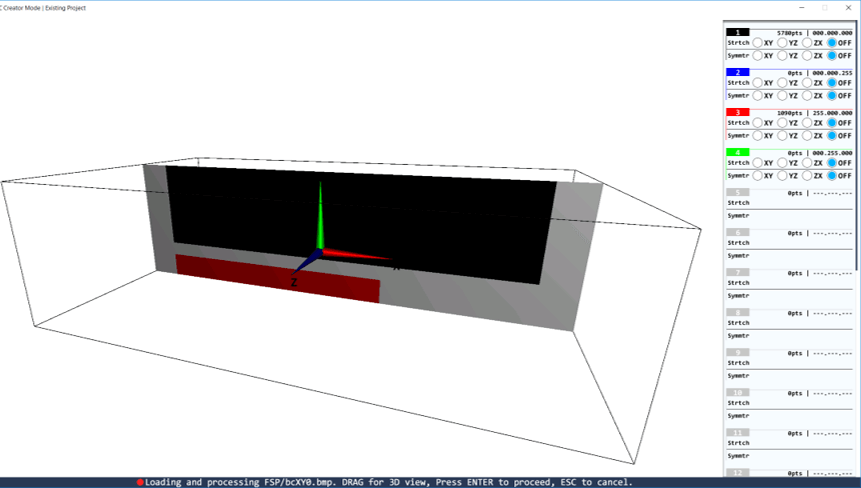
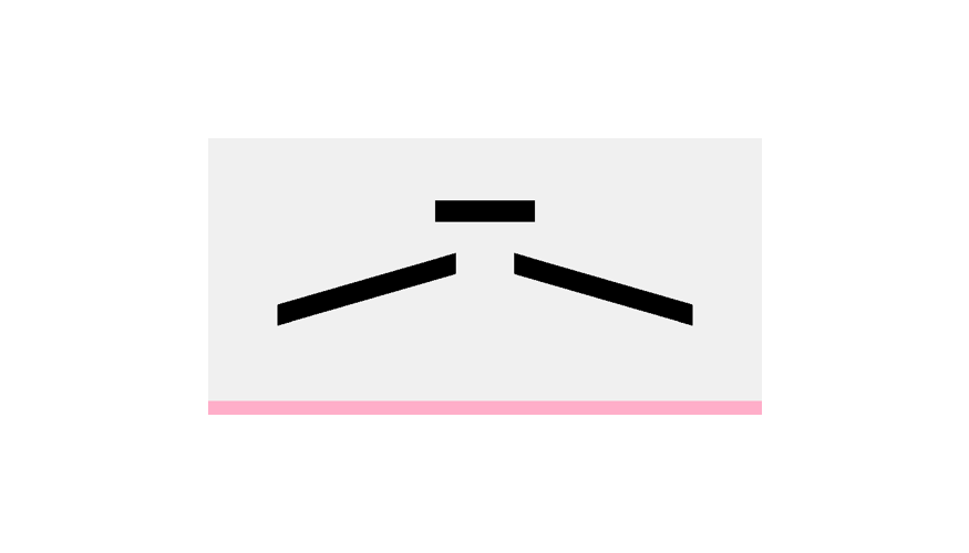
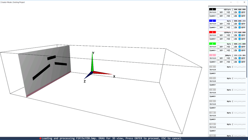
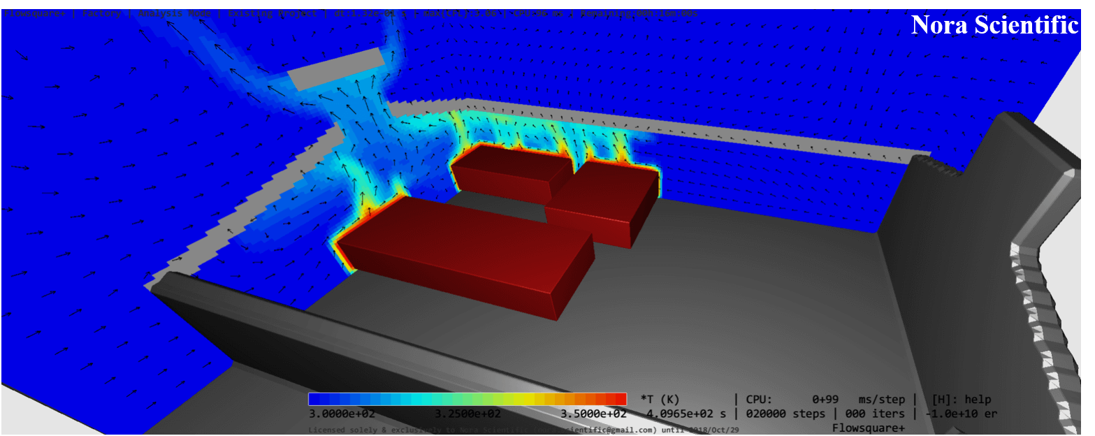
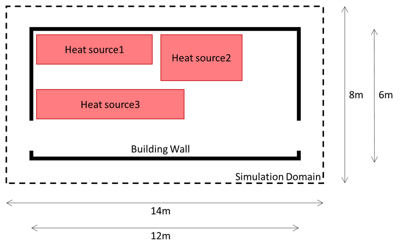
In this simulation, we will consider a air flow in a building where there are three heat sources with the same temperature. There are (small) openings both sides (X-direction) of the building, and top of the roof, as shown in the below 3D and schematic figures.
The building design is intended to let the heated air go out from the open slits on the roof, while the outside air come in from two openings on the sides (of course, this design concept needs to be verified with the present simulation!).
The initial (inside and outside of the building) air temperature is taken as 300 K (27 degree C), and the temperature of the heat sources is 350 K (70 degree C). All walls are assumed to be adiabatic.

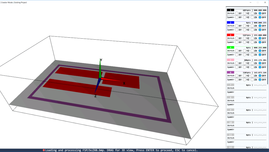
3. Construction of Simulation Domain
General rule of constructing 3D boundary conditions is explained in here.
In this simulation, we will specify:
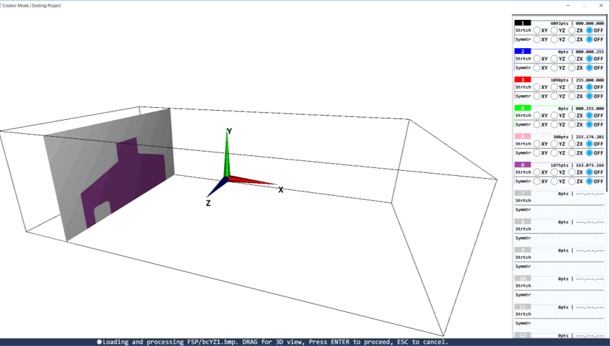
- the building side walls (NON-preset color, magenta)
- the floor/ground (NON-preset color, pink)
- the heat sources (preset color, red)
- the roof (preset color, black).
All of these four parts are constructed by using "(b) Model constructed by third angle projection".
The paint image pixel sizes can be irrelevant to actual physical domain dimensions. However, it is a good habit to use more or less similar aspect ratio between images and domain dimensions. In the present example case, 1m length corresponds to 100 pixels in the paint images.
4. Simulation Parameters
Several important parameters are explained here. More thorough information about parameters can be found here.
- cmode
cmode is taken as 1 for the 1:Thermo fluid simulation mode (varying temperature ideal-gas flows). - lx The domain length in X-direction is 14m.
- ly The domain length in Y-direction is 4m.
- lz The domain length in Z-direction is 8m.
- nx、ny、nz The number of mesh points needs be determined based on the required spatial resolution. Here, we will use (nx, ny, nz) = (200, 50, 100). The thinnest part of the 3D model (in this case, perhaps wall) should be resolved by few mesh points at least, unless the part is on the computational boundary.
- tempW
Initial air temperature is set to be 300K. - vinW
Initial Y-direction (vertical) velocity component is taken as -0.1m/s. This is a little trick for a stable simulation: Flowsquare+ determines initial time step size automatically, which depends on initial velocity magnitude, which requires non-zero initial velocity at some region in the domain. Artifact of this procedrue does not influence the solution as long as the simulation is run long enough. - uinR、vinR、winR
The heat sources are solid, and this red "inflow" boundary should be treated as the solid wall, uinR = vinR = winR = 0 m/s. Since these value is default value for these parameters (see here), these parameters do not need to be specified explicitly in the parameter editor. - tempR
The temperature of the heat sources is 350K. - tempWallK
The roof specified by the black color is an adiabatic wall, so tempWallK=0. - tempWall
The bulding side wall and floor/ground, specified by NON-preset color, are adiabatic too, so tempWall=0. - gfy
To include the effect of the gravity (thereby natural convection), gfy = -9,8 m/s^2 (minus means downwards).
5. Simulation
Using the input files provided in the above link, you can perform the simulation with these steps, and obtain solution similar to the following images!
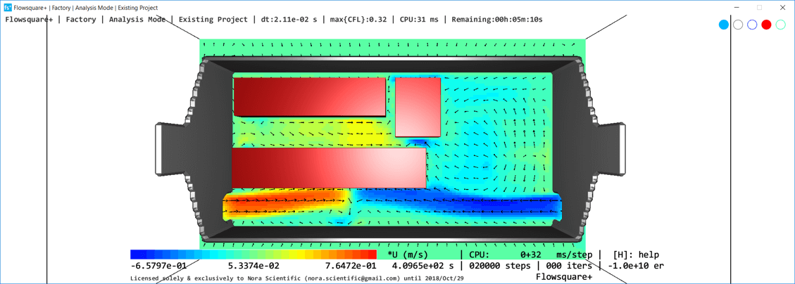
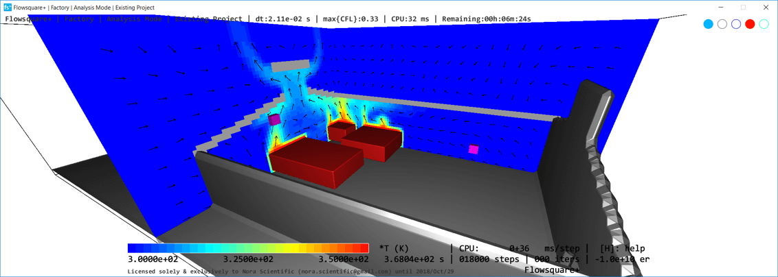
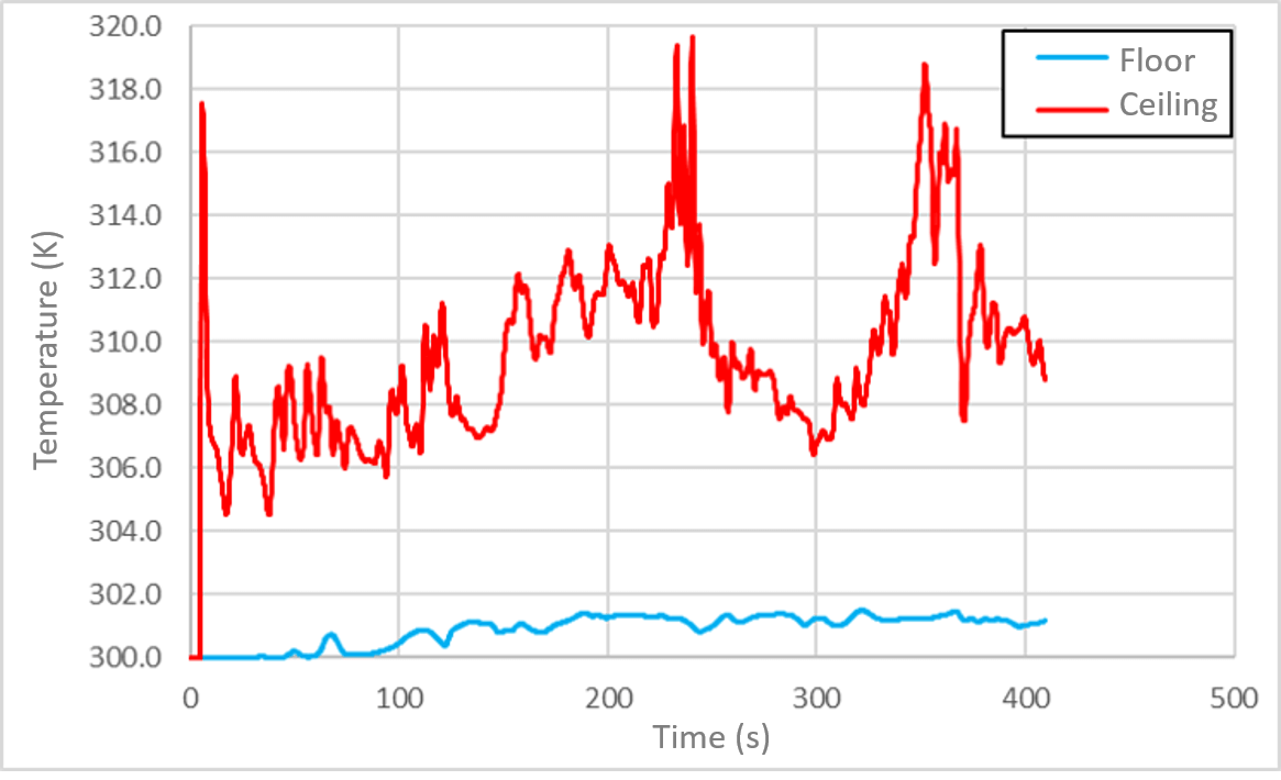
You can also measure temporal temperature and air flow evolutions by using probes. The below figure shows temperature evolution measured at the two probes, one near floor and the other near the ceiling shown in the above figure. You can add a ventilation in the configuration for better cooling performance, and check that out with Flowsquare+!
 JP
JP