The Easiest Computational Fluid Dynamics Software
 JP
JP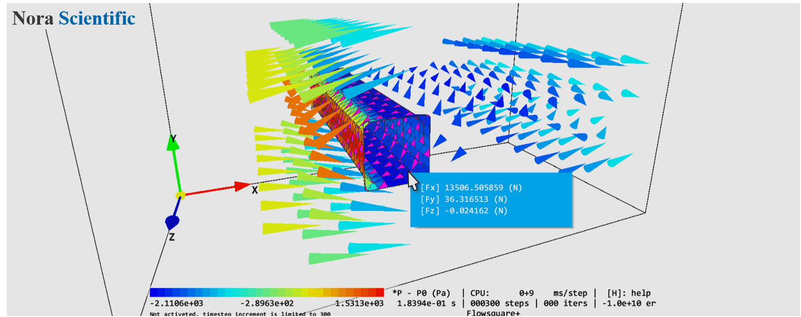
Flowsquare+ for Beginners
Introduction
Here, we will demonstrate how to perform a typical fluid simulation with Flowsquare+ by using test case input files which are also included in the Flowsquare+ download file. The test case is set up for a simulation of Karman vortex street. There are only 10 steps to follow to perform your first simulation!
This page explains for newer versions of Flowsquare+, 2021R2.0 or later. For older versions (2021R1.0 or earlier) visit this page.
- Simulation steps
- 1. Installing Flowsquare+
- 2. License activation (skippable)
- 3. Setting project name
- 3a. (Loading an existing project)
- 4. Setting input file path (only for a new project)
- 4a. Create input files from scratch (for a new project)
- 5. Project confirmation
- 6. Project file structure
- 7. Parameters loading and setting
- 8. Loading boundary configuration images
- 9. Comfirming constructed boundary
- 10. Starting your first simulation!
(tracer particles and XY color contour).
1. Installing Flowsquare+
You can download Flowsquare+ from here. You need to accept the license agreement and disclaimer to do so.
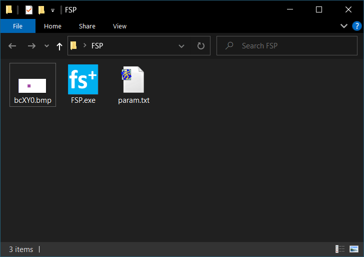
Then, you need to Unzip the downloaded file by selecting "Extract All", and make sure you have the below files in the FSP folder (below figure).
- FSP Folder
- FSP.exe (executable file)
- bcXY0.bmp (input file; boundary configuration image file)
- param.txt (input file; parameter file)
Now Flowsquare+ is ready to use!
2. License activation (skippable)
Let's double click FSP.exe and execute Flowsquare+. License key input field is diplayed first, but this can be skipped for now. Press [Enter] key or  to proceed. To cancel, press [ESC] key or
  .
.
3. Choosing project
* Project folder save location is no londer constrained in 2021R2.0 or later.In this step, we specify a new project to create or existing project to load. In this example, we will create a new project.
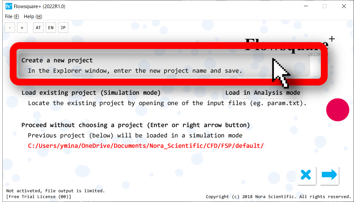
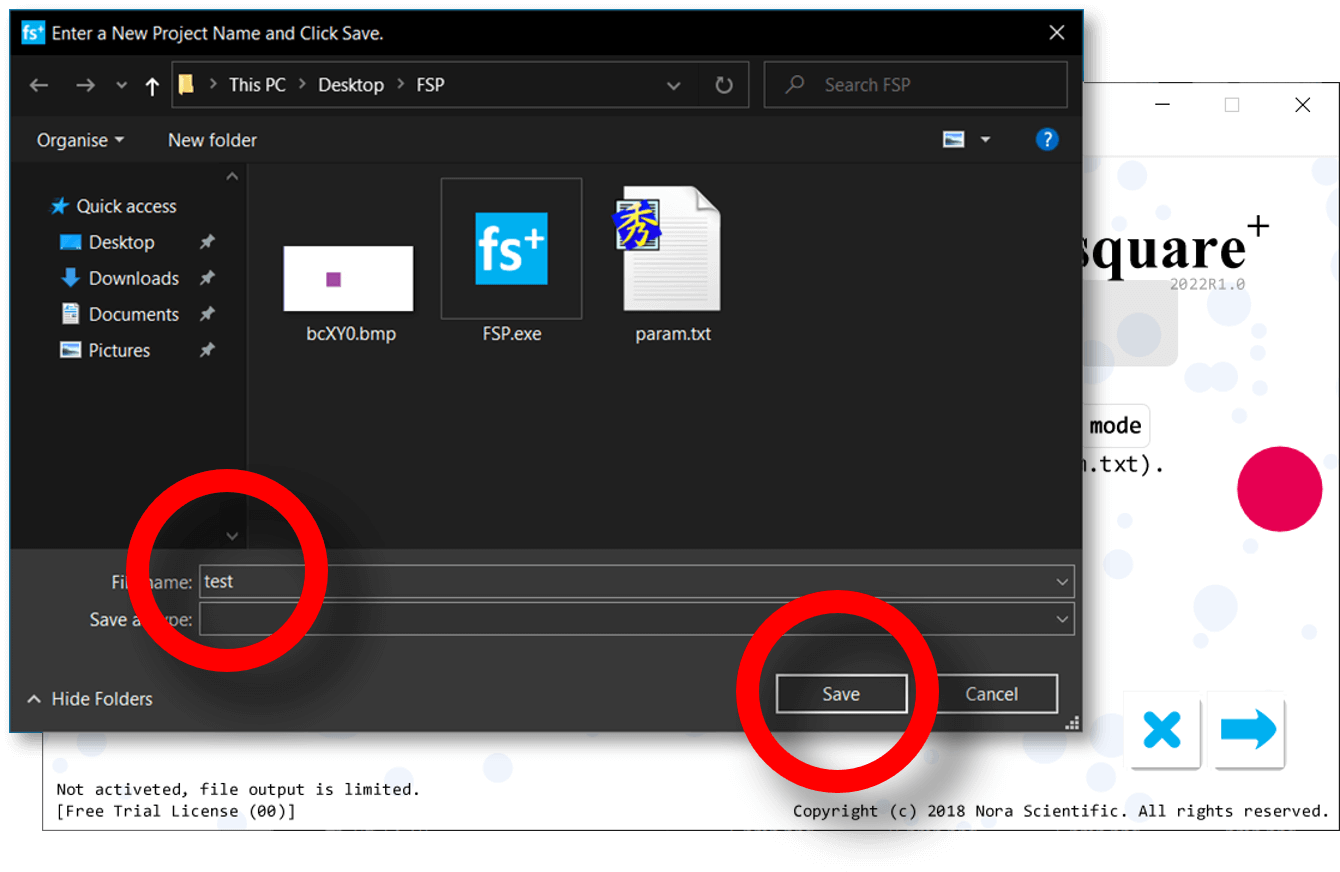
By clicking "Create a new project" (red box above figure), a file explorer opens. Navigate to the location you want to save the project folder, enter a (new) project name (left red circle below), and click on Save button (right red circle in below).
In this example, a new project "test" is saved in the FSP folder stored under the Desktop.
3a. Loading an existing project
To load an existing project, choose "Load existing project", and open one of input files in the project (eg. input/param.txt) in the file explorer. When opening an existing project, select an execution mode:
- Simulation mode
For a new simulation or resuming a simulation. A new project is always opened in the simulation mode. - Analysis mode
For visualization and analyses of output (dump) data from a previously completed simulation.
4. Input file path (for a new project)
For a new project, you will choose input files to be copied to your new project.
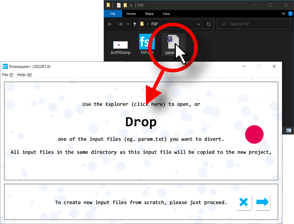
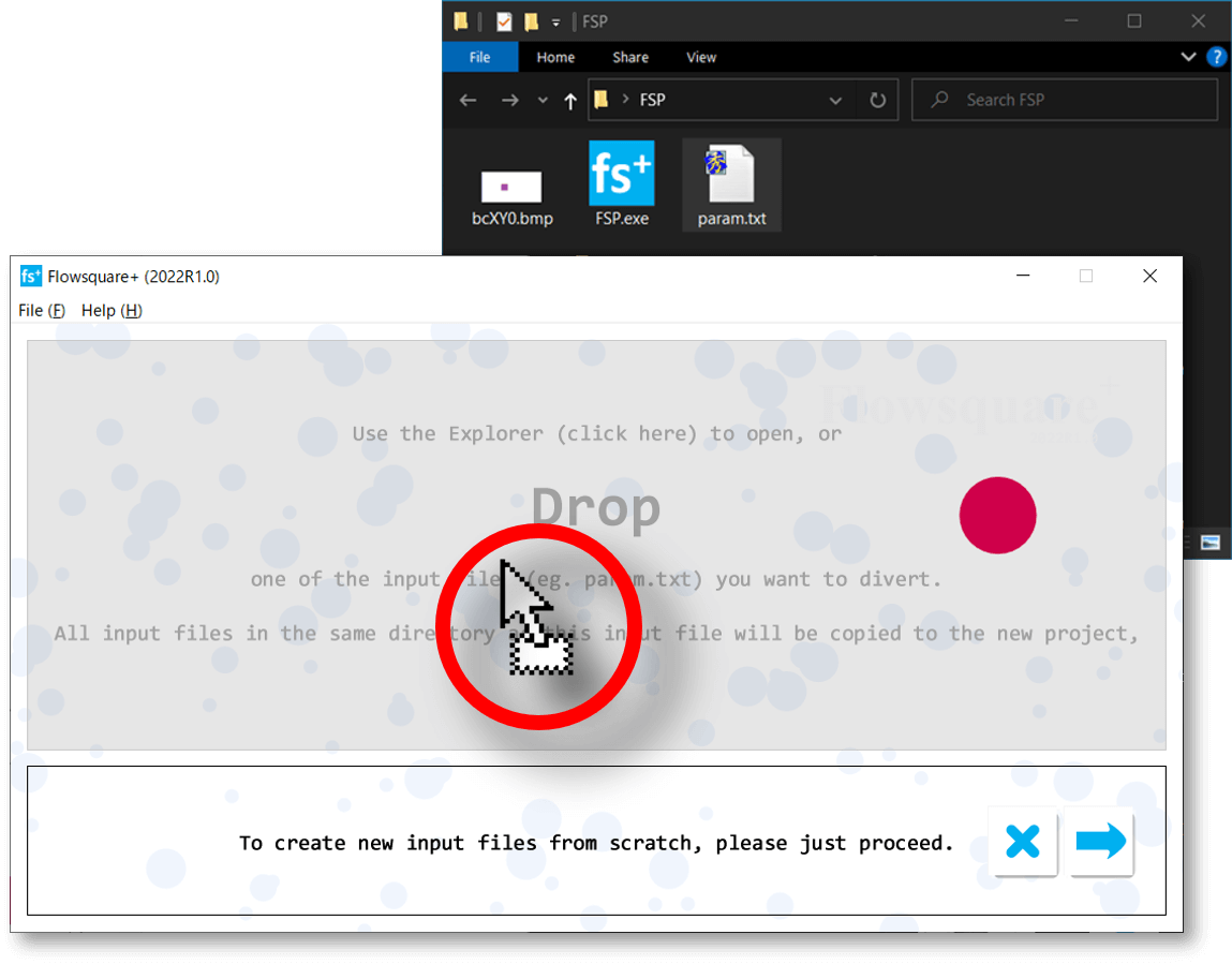
You can just drag & drop one of the input files to set the file path of source input files. Or, by clicking the window, you can choose one of input files in the file explorer. All input files in the same directory as selected input file will be copied to the new project.
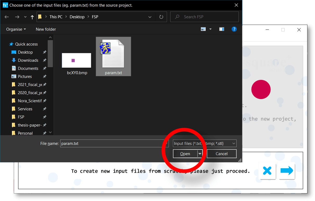
Proceed to the next without choosing a file, input files will be copied from the previously loaded project.
In this example, we drag&drop the default param.txt file in the FSP folder as in the red arrow/circle in below figure. For an existing project, all input files in input folder in the project folder will be loaded.
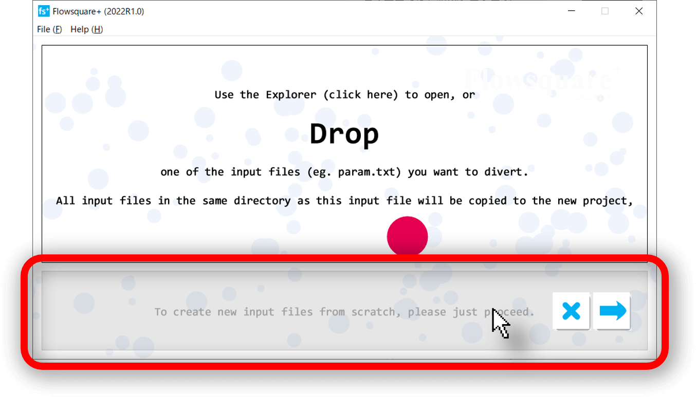
4a. Create input files from scratch (for a new project)
You can create your own input files from scratch, rather than copying existing input files as explained above. To do so, just proceed to next ([Enter] key or ), or click the highlighted area in the below figure. After the project confirmation window described next, you can create and edit input parameters and input bmp images in the parameter editor window.
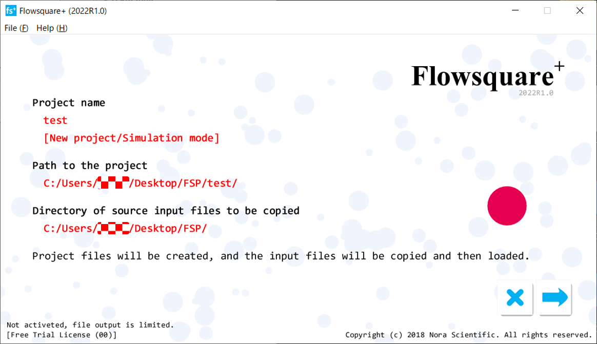
5. Project confirmation
Now, let's confirm the blow project configuration.
- Project name
test - Project status
a new project, or an existing project - Execution mode
Simulation mode, or Analysis mode - Project folder location (absolute path)
(Eg.) C:/Users/.../Desktop/FSP/test/ - Location of source input files (absolute path) *only for a new project
(Eg.) C:/Users/.../Desktop/FSP/
Once confirmed, press [Enter] key or to proceed. To cancel, press [ESC] key or . Now, a new project folder will be created in the specified location, and all the input files are copied onto the project folder.
6. Project file structure
All projects in Flowsquare+ have following project file structure. All project files are stored in a project folder.
As an example, a project file tree is shown below for the project "test" created above.
- test: a project folder
- dump: a folder for simulation result data
- figs: a folder for simulation figures
- input: a folder for all input files
- input file #1
- input file #2
- ...
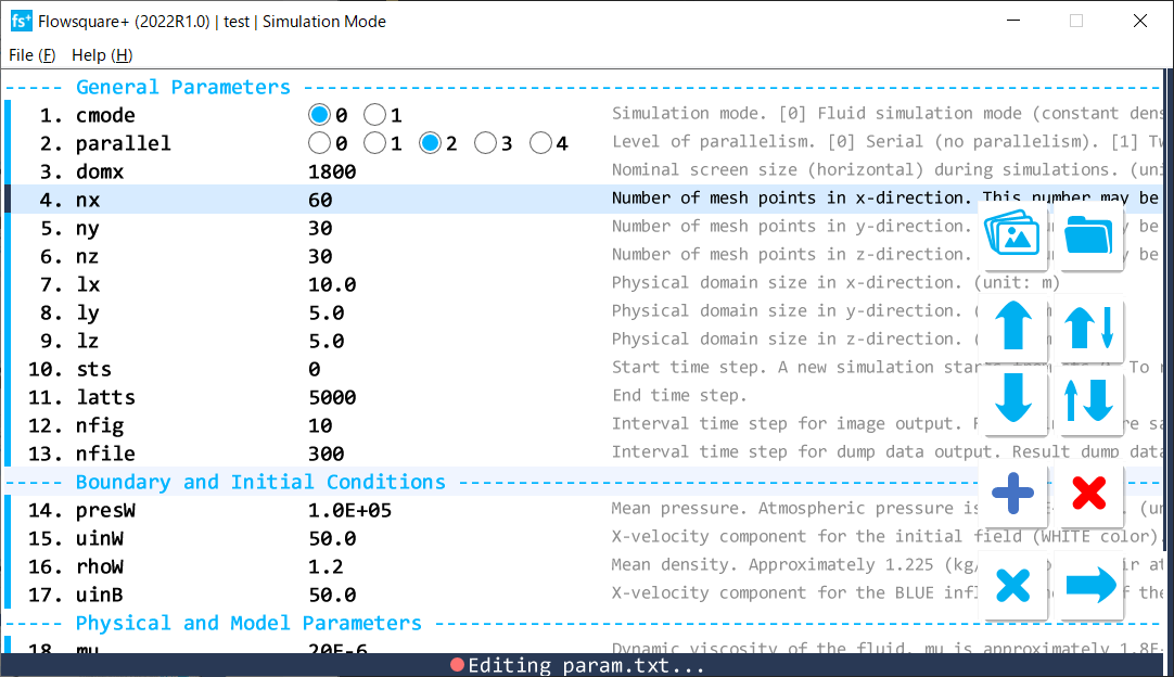
7. Parameter loading and setting
Once the project folder is created successfully, the parameter file, param.txt is loaded from the project folder. The parameter file defines all the parameters related to the simulation. The parameter file is displayed in the parameter editor, in which you can modify each parameter value, and also add  , remove
  , rearrange
  /
/ parameters, because many of tunable parameters may not be necessary for your simulation.
If the simulation mode is used, any change in parameters will be saved at this moment. For the analysis mode, no change will be saved.
For the present case, no parameter needs to be changed, so please press [Enter] key or to proceed.
8. Boundary configuration images
Next step is to load boundary configuration images (if any). In this step, boundary configuration images (BMP images whose name begin with "bc") are loaded from the project folder one by one, and each of them is displayed with the discretization mesh defined in the parameter setting as follow.
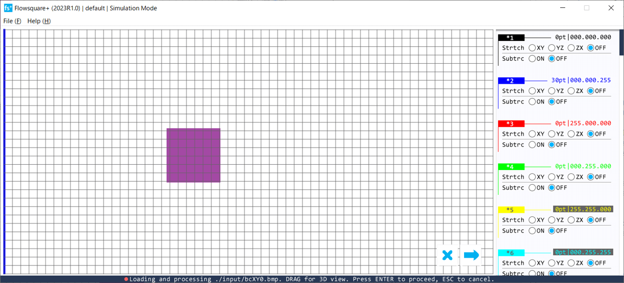
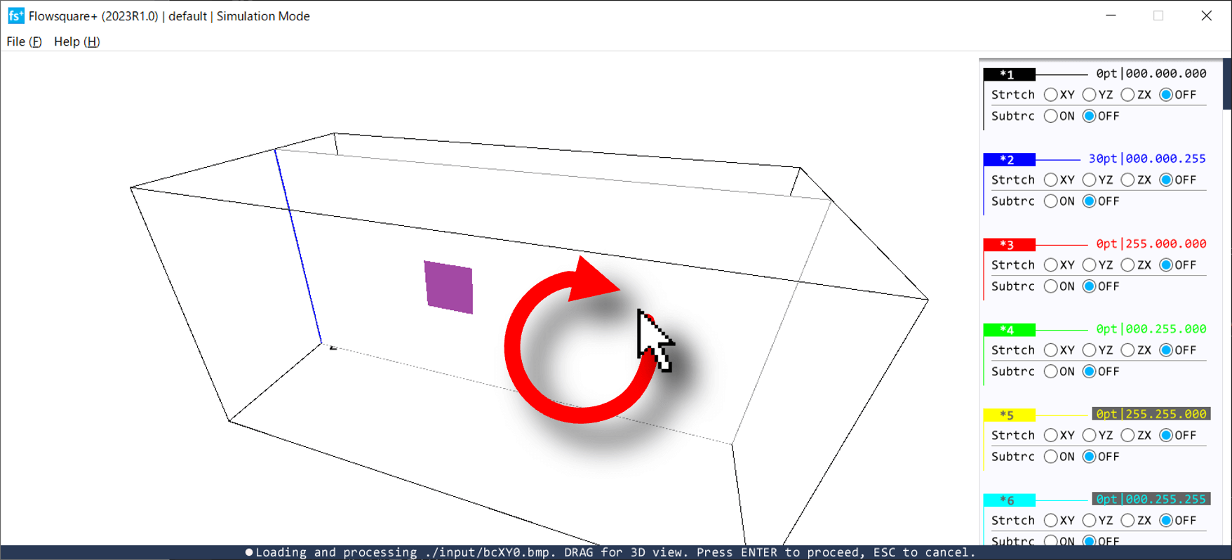
With a mouse drag operation in the domain area, you can see the direction of the boundary configuration image in the 3D field from any direction as in below figure.
This step also allows you to specify advanced configuration options such as "Stretching", "Symmetric" and "Inverse". If there are more than one configuration images, pressing [Enter] key or loads the next image. If you have a CAD (STL) model to use, it will be loaded after all images are loaded.
There is only one image and no option will be needed this time, so please press [Enter] key or to proceed. Boundary construction will be started.
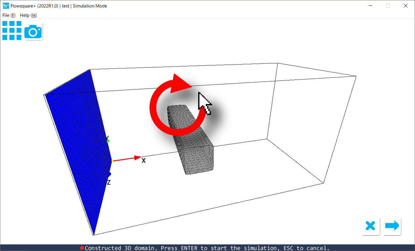
9. Constructed boundary and simulation domain
Finally, constructed boundary and simulation domain are visualized so you can confirm whether they seem good. You can perform various mouse/keyboard operations to view your simulation domain from various angles and distance. If you are happy with the domain and boundary configuration, press [Enter] key or to proceed. To cancel, press [ESC] key or . Your first simulation will be started immediately!
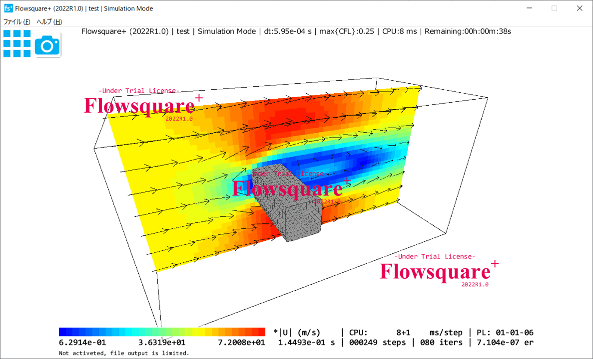
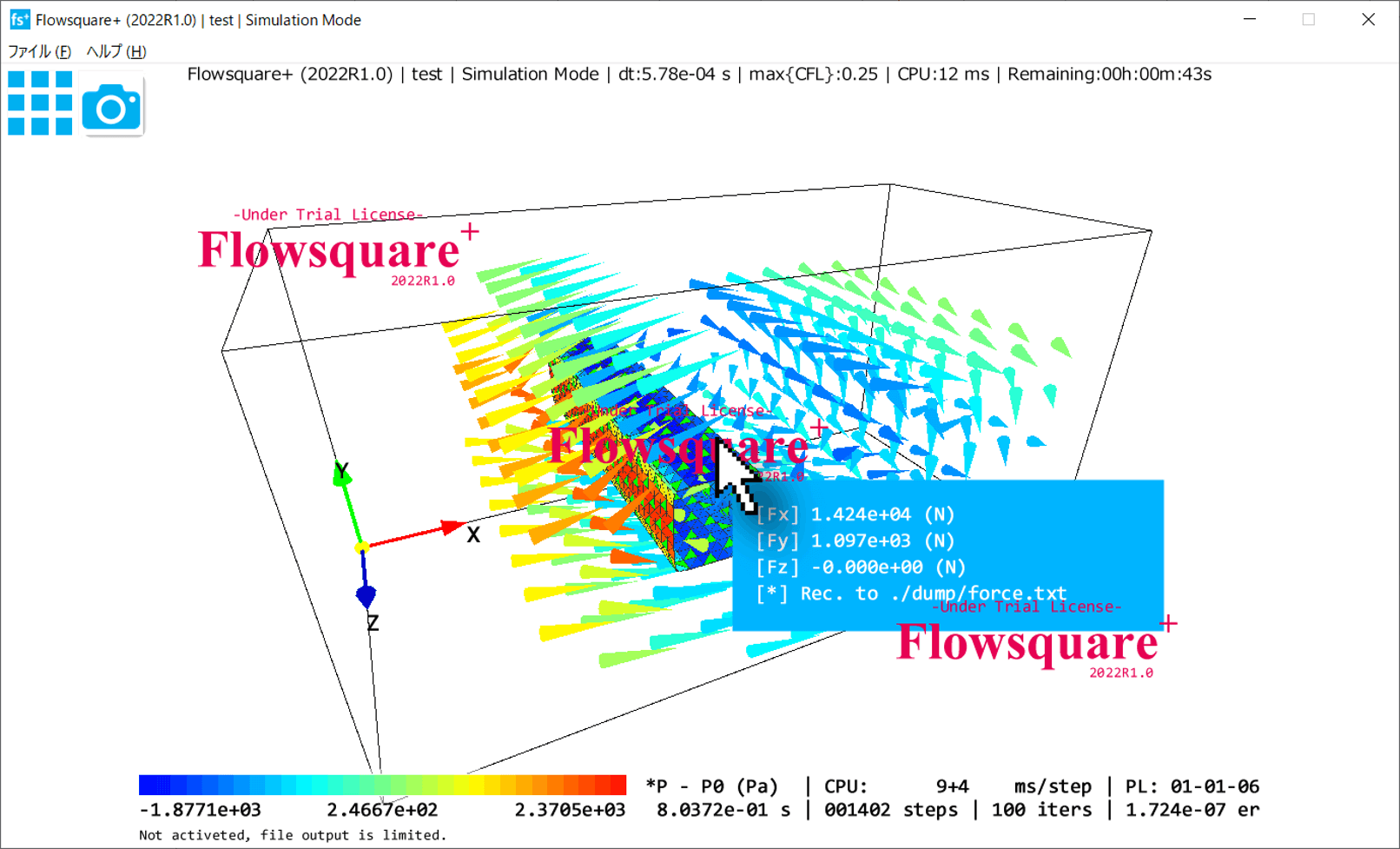
10. Your first simulation!
Once the simulation has been started, visualization of the flow field is performed in-situ at the same time as computation. There are various tools in Flowsquare+ to visualize the flow field.
Simulation images are saved once in every nfig time steps, and instantaneous solution data (field data; dump data) are saved once in every nfile steps. Here, nfig and nfile are parameters specified in the set of parameters. These images and dump data are respectively saved in figs and dump folders in the project folder.
The saved images can be used to generate a movie of your simulated flow after simulation. Also, the saved dump data can be loaded by using the analysis mode to examine the simulated flow field closely using many analysis tools provided in the Flowsquare+.
The free trial license we used for this case limits the file output beyond 300 steps (2020R1.0 or later). For more useful simulation and analysis, please consider using a professional license.
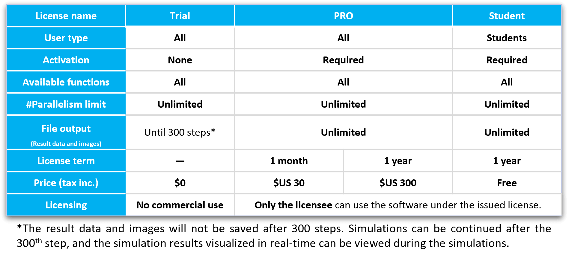