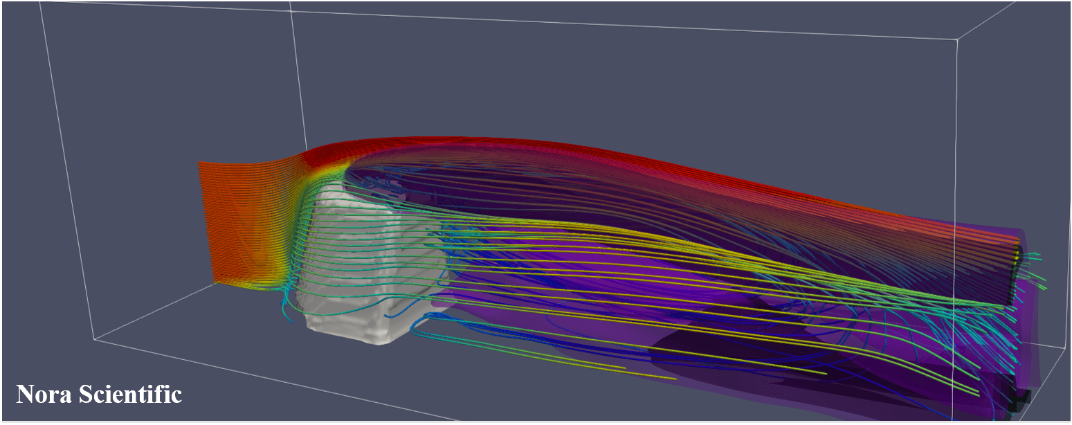
Visualization using Paraview

Visualizing Flowsquare+ simulation results using external tool

1. Introduction

Paraview is an open source scientific visualization software developed by Sandia National Laboratories and others. Although Flowsquare+ has several basic visualization tools, Paraview can generate more beautiful and insightful visualization image.

The title image of this page is a Paraview visualization example of an example simulation "Air Pollution on Cruise Ship Decks". Paraview includes variety of visualization and analysis tools, only parts of which are explained in this tutorial.

---

 

2. Installation and execution of Paraview

You can download Paraview from https://www.paraview.org/download/.

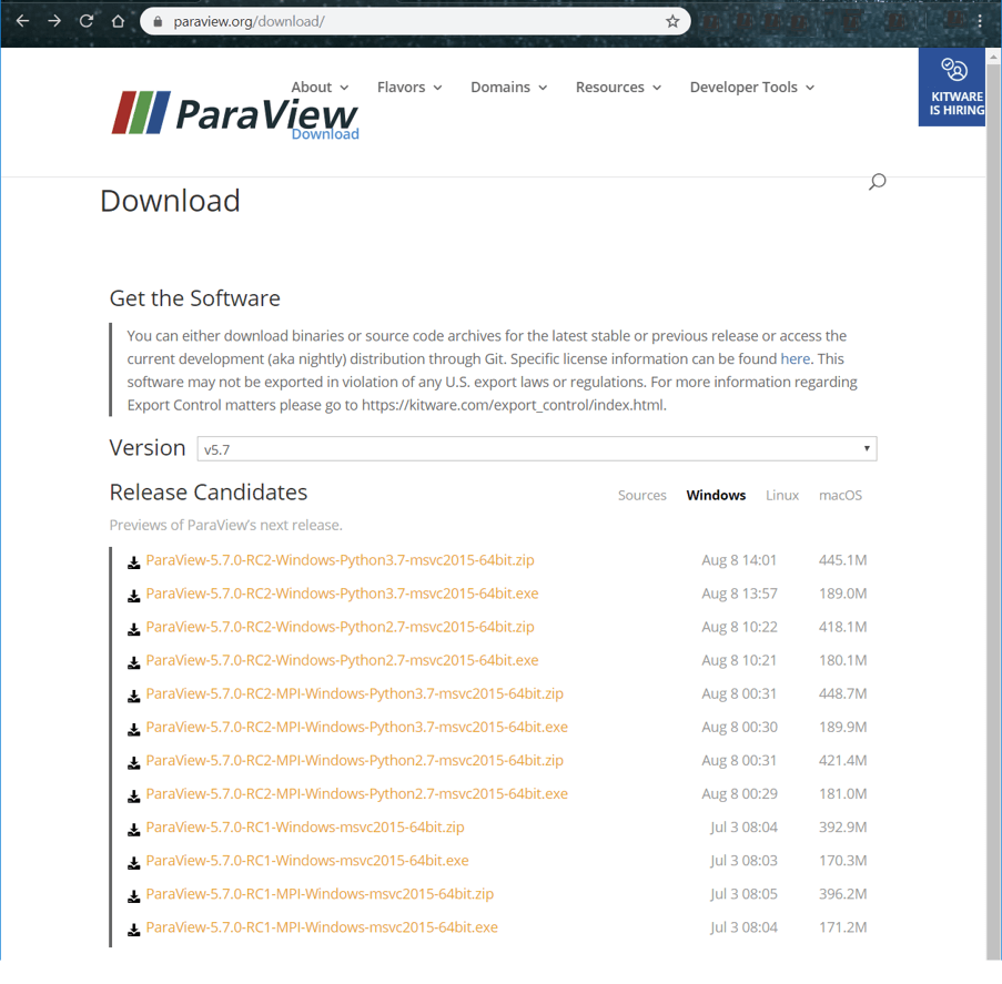
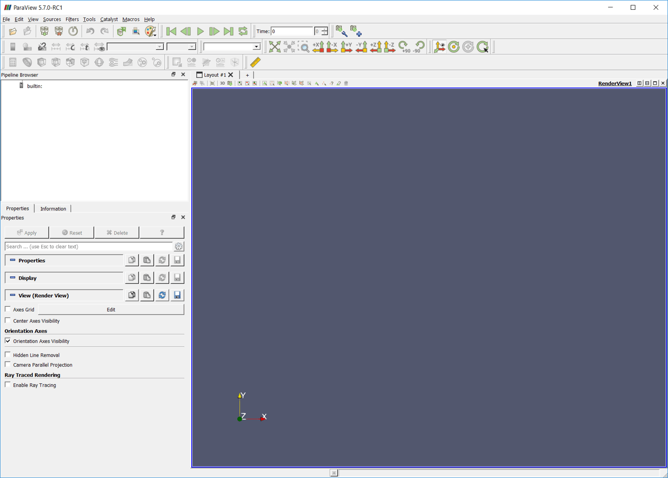
There are several releases for the same version. The latest as of today (26/Aug/2019) is v5.7, and we will download "ParaView-5.7.0-RC1-Windows-msvc2015-64bit.exe" here. If you are not sure which file to download, download the one does NOT contain "Python" and "MPI" in their file names. Also, please download one with *.exe extension. After download, please execute the downloaded *.exe to install Paraview. Once installed, start Paraview from the Windows menu, which looks like below figure.

---

 

3. Loading Flowsquare+ result files

Loading Flowsquare+ results file into Paraview is easy. In the menu bar, click [File]→[Open] to open a file window below. Navigate to the Flowsquare+ directory.

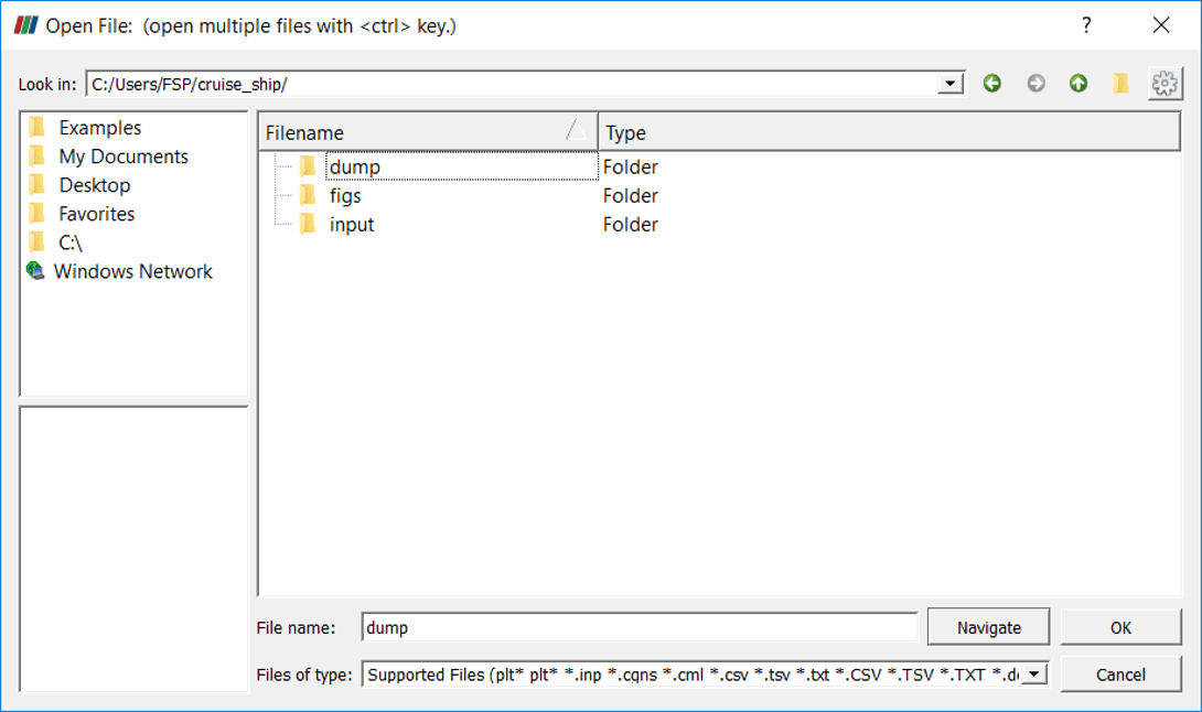
In Flowsquare+, all output files are stored in dump directory under each project directory. In the dump direcotry, there is a sub-directory for each timestep. In the timestep sub-directory, instantaneous field data are stored as explained in here, and eqch physical field is saved in an individual file.

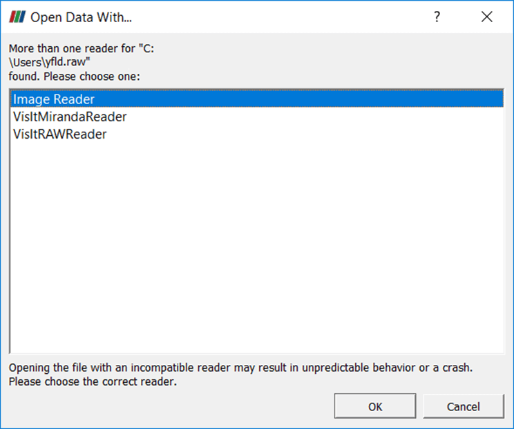
Here, let's open the pollutant mass fraction field (yfld.raw) at 10000-th timestep (in 00010000 directory under dump) from the example simulation "Air Pollution on Cruise Ship Decks". The following window appears to choose a file type, so select "Image Reader" and click "OK".

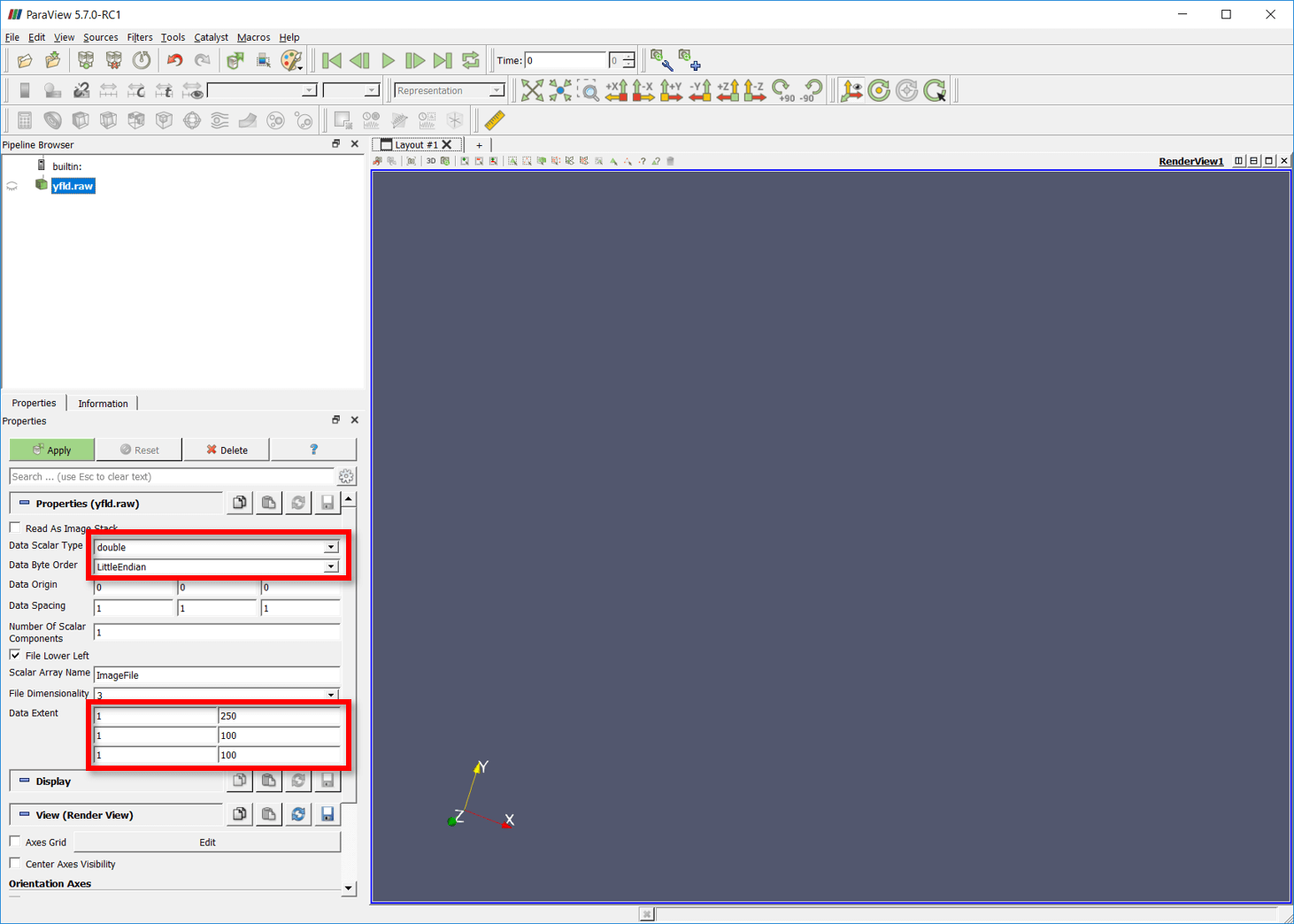
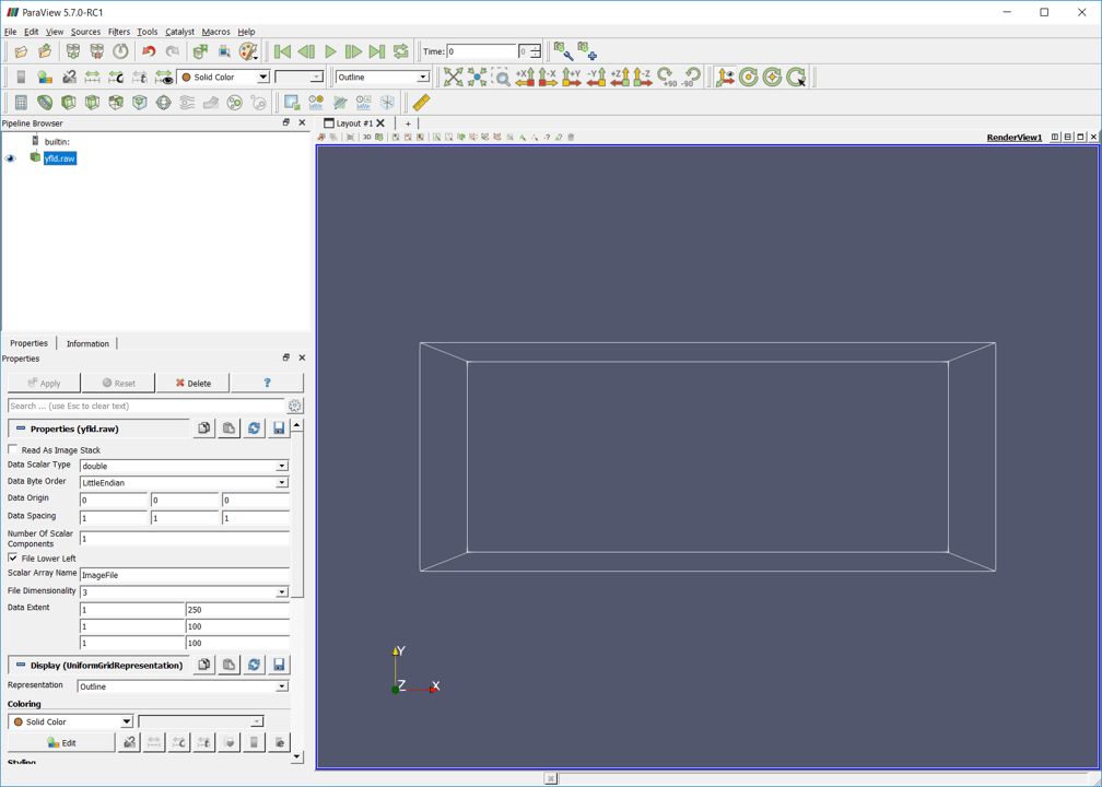
We then need to set data specification. Set "double" for "Data Scalar Type", and "LittleEndian" for "Data Type Order". "Data Extent" corresponds to the beginning of mesh point (1) and number of the mesh point for directions \((x, y, z)\) from top to bottom, which are essentially \((nx, ny, nz)\) of the simulation. By default, these parameters are set to be 0 (zero) in Paraview, so please do not forget to change these values. After setting these values, click "Apply" to start loading the data (it may take some time). Once loading is complete, the outline of simulation domain is typically displayed.

---

 

4. Visualizing loaded Flowsquare+ data

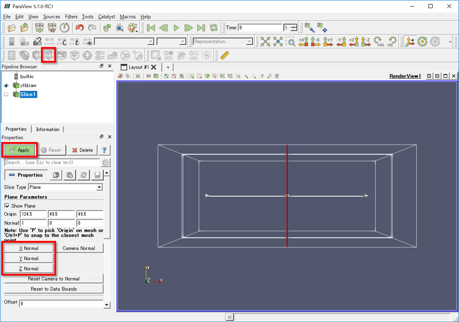
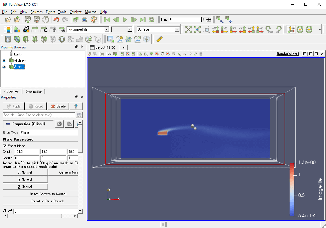
Now, we would like to visualize the loaded pollutant field data in a two-dimensional cross-section color contour. Click "Slice" button highlighted in a red box below. A slice property window appears bottom-left of the Paraview window. In the property window, there are "X Normal", "Y Normal" and "Z Normal"buttons, and they are to display a 2D slice normal to \(x, y,z\)-direction, respectively. Here, let's choose "Z Normal", and click "Apply" button. Paraview displays 2D color contour of pollutant distribution using a default setting.

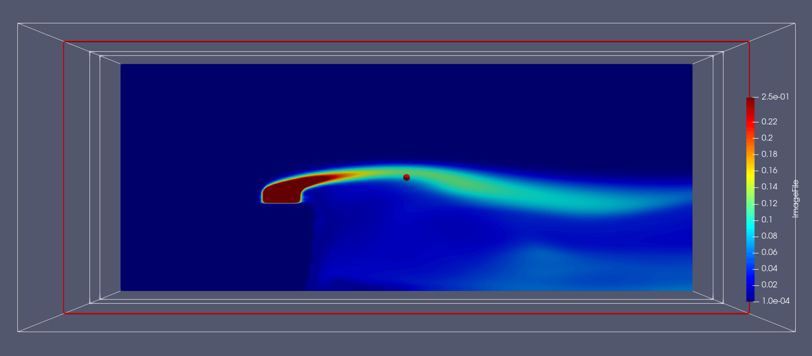
The default setting does not look too great. In such case, you can modify verious visualization setting. In the property window, these buttons can be used to (from the left) set color scale (auto), color scale (manual), scaling based on entire times, colormap. Below image shows just an example of how the same result looks like with a different setting.

---

 

5. Vectorize Flowsquare+ data

All the physical quantities considered in Flowsquare+ are saved in separate files, which includes velocity vector field \(u, v, w\). Here, we will describe how to construct a vector field from three separate vector component files.

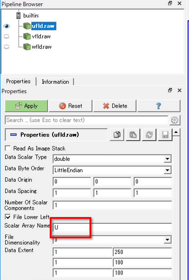
First, load these three velocity component data (\(u,v,w\)) following directions above. These files are respectively ufld.raw、vfld.raw、wfld.raw. Also, in the property window, set an appropriate name for each field, by setting "Scalar Array Name", which is "ImageFile" by default. For example, ufld.raw could have name such as "U" (field name setting example.). After putting a name, click "Apply" button. Repeat this procedure for the two other velocity component (V and W).

After loading all, select these three fields. You can select multiple fields by mouse clicking while pressing a Ctrl key.

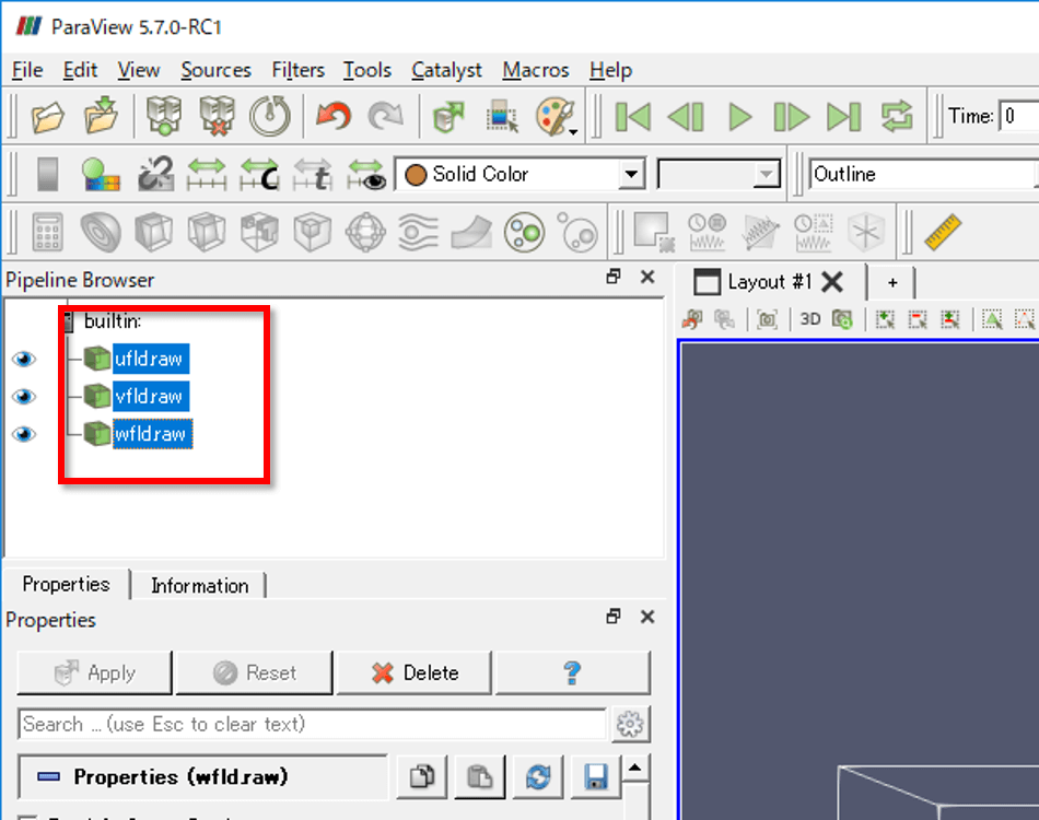
After selecting all the velocoty component, click through "Filters"→"Alphabetical"→"Append Attributes" from the menu. There will be AppendAttributes in the pipeline browser. Click Apply.

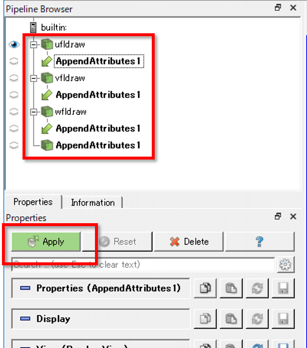
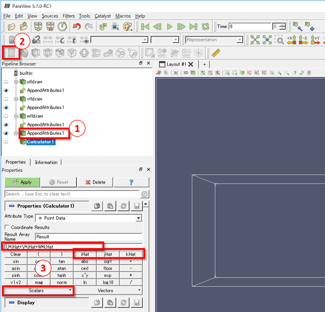
Select the bottom "AppendAttributes1" (1 in the below image), and then click the Calculator icon (2 in the below image). There will be a new property in the below. Write U*iHat+V*jHat+W*kHat in the equation field (3 in the below image), where U, V and W are the name of velocity components set above. You can also set this equation by using displayed buttons and pull-down menu (3 in the below image). Finally, click Apply, and velocity vectors are stored in the "Calculator1" in the Pipeline Browser.

---

 

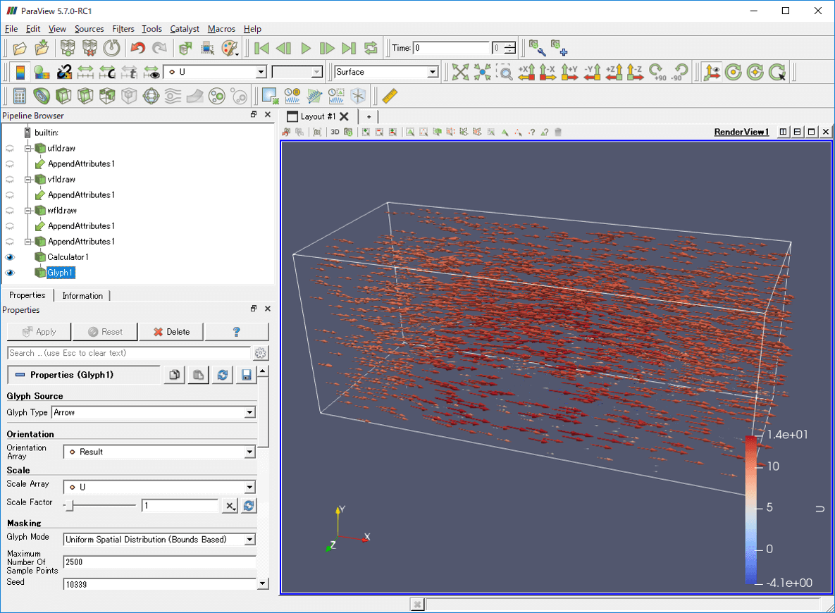
6. Visualizing vector field

Now let's visualize the vector field we created above. Select the vector data we just created in the pipeline browser (here the name is Calculator1). Then, use Glyph (vector arrow) or Stream Tracer (streamline) to visualize vector fields. These visualization tools have their own setting parameters (e.g. length, width, numbers) which you may want to adjust. The below image is an example of velocity vector visualization using Glyph. Also, the title image of this page is another visualization example using Stream Tracer (overlaid on some iso-surface).

---

 

---

Top