The Easiest Computational Fluid Dynamics Software
 JP
JP
Simulation Parameters
Introduction of Flowsquare+ parameters
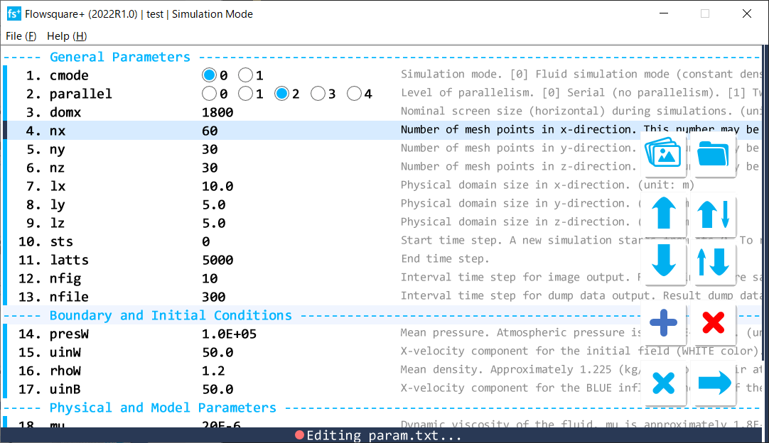
All parameters relevant to computation in Flowsquare+ are set up in the Parameter Editor and stored in param.txt.
All the dimensional parameters are specified in SI units (mentioned in the list below). Also, [...] next to each parameter name denotes the default value of the parameter. If a parameter is not set by the user, and is necessary for the simulation, this default value is used throughout the simulation. There is no specific order in which parameters need to be specified, and you do not have to specify all the parameters listed below. You can add, delete, change the order of parameters in the Parameter Editor as described here.
Users can refer to the parameter setting of example cases for their simulations. For more suitable parameter setting, it's good to understand their physical meanings. The following parameter list describes all the parameters, their physical meanings, and optimal values.
List of available parameters
[Note] For a parameter whose name is followed by ** in the below list, you can specify " - " (hyphen) as a parameter value instead of a number. Such a parameter does not constrain a corresponding quantity at corresponding locations. For example, on the computational boundary points, a slip boundary can be specified by setting "-" for wall tangential velocity components as inflow condition. Or you can specify scalars (temperature, mass fraction and/or age variable) on the boundary without modifying the velocity field.
Also, setting a magenta boundary in the domain, and setting non-magenta inflow boudary's temperature and/or mass fraction values as " * " (asterisk) as an input, the corresponding quantity at the corresponding boundary is set as the volume averaged value within the magenta boundary (feedback). In such a case, all the quantities at the magenta boundary is set as " - " (non-constraint condition for all quantities).
- cmode [0]
Simulation mode. An option is chosen from radio buttons.- Fluid simulation mode (constant density, constant temperature, single phase for gas and liquid flows)
- Thermo fluid simulation mode (varying temperature ideal-gas flows)
- ageFlag [0][2021R1.0 or later]
Whether including the age variable transport equation during simulations (ageFlag=1) or not (ageFlag=0). - parallel [0]
Level of parallelism. An option is chosen from radio buttons. npx, npy, npz are automatically allocated.- Serial: no parallel computation
- Two: #parallelism = 2
- Low: #parallelism = max(1, maxThreadsAvail / 4)
- Med: #parallelism = max(1, maxThreadsAvail / 2)
- High: #parallelism = maxThreadsAvail
*maxThreadsAvail: maximum #threads determined by the system.
- nprocs [none][2020R1.0 or later]
Level of parallelism. You can specify any number of threads less than "maxThreadsAvail", which cannot be chosen by parallel above. If nprocs is specified, the choice in parallel is ignored. npx, npy, npz are automatically allocated. - npx [none][2020R1.0 or later]
Level of parallelism allocated for x-size of the simulation domain. npx has to be specified along with npy and npz. If npx, npy, npz are specified, nprocs = npx * npy * npz regardless of nprocs input above. - npy [none][2020R1.0 or later]
Level of parallelism allocated for y-size of the simulation domain. npy has to be specified along with npx and npz. If npx, npy, npz are specified, nprocs = npx * npy * npz regardless of nprocs input above. - npz [none][2020R1.0 or later]
Level of parallelism allocated for z-size of the simulation domain. npz has to be specified along with npx and npy. If npx, npy, npz are specified, nprocs = npx * npy * npz regardless of nprocs input above. - ibm [1][2019R1 or later]
Boundary specification method. An option is chosen from radio buttons.- Conventional grid-wise boundary condition
- Immersed boundary method
- domx [1024]
Nominal horizontal window size during simulation (pixel). 1600 pixels or larger is recommended. - nx [1]
Number of mesh points in x direction. nx can be set independently from the domain size aspect ratio. - ny [1]
Number of mesh points in y direction. nx can be set independently from the domain size aspect ratio. - nz [1]
Number of mesh points in z direction. nx can be set independently from the domain size aspect ratio. For 2D simulation, nz=1. - lx [1.0]
Simulation domain size in x direction (m). - ly [1.0]
Simulation domain size in y direction (m). - lz [1.0]
Simulation domain size in z direction (m). - sts [0]
Time step of the beginning of a simulation. A new simulation starts with sts=0. To restart a simulation, sts is the time step at which you restart the simulation from. Note that dump data needs to be generated at this time step in the previous simulation. See nfile below. - latts [300]
Time step of the end of a simulation.
- cfl [0.1]
A CFL number. A CFL number is used to determine time step size (Δt). Flowsquare+ monitors maximum CFL number, and dynamically adjust the time step size so that the CFL number always stays close to the value set in cfl. For most cases, cfl = 0.2-0.3. - deltat [none][2020R1.0以降]
Time step size (Δt) (s). If deltat is set, Δt is no longer adaptively determined based on cfl, and a constant value of deltat is used. - nfil [0]
Frequency of spatial filtering to be used when simulation becomes numerically unstable. Set 0 when not used. Spatial filtering is performed once in nfil time steps. - wfil [0.0]
Nondimensional weight of the spatial filtering (0.0≤wfil≤1.0). Solution from simulation being qraw and fully-filtered value being qfil, the final solution is calculated as q = wfil * qfil + (1 - wfil) * qraw. - npfil [1][2019R2 or later]
Frequency of spatial filtering for pressure field to be used when simulation becomes numerically unstable. Many simulations performed by using Flowsquare+ lacks resolutions to resolve physical boundaries, and this often cause unphysical pressure oscillation. Set 0 when not used. Spatial filtering is performed once in npfil time steps. - wpfil [0.5][2019R2 or later]
Nondimensional weight of the spatial filtering (0.0≤wpfil≤1.0). Solution from simulation being praw and fully-filtered value being pfil, the final solution is calculated as p = wpfil * pfil + (1 - wpfil) * praw. - peps [1.0e-6]
Residual error tolerance of the iteration calculation for the Poisson's equation (relative error respect to presW). The iteration calculation is terminated even if error is greater than peps when the number of iterations reaches loopmax. - omega [1.8]
A relaxation parameter in the SOR method for the Poisson's equation. Typically 1.8 is used, but a smaller value may be used when a simulation keeps diverging. - loopmax [1000]
Maximum number of iterations for the Poisson's equation. The iteration calculation is terminated even if error is greater than peps when the number of iterations reaches loopmax. - presW [1.0e+5]
Initial pressure (Pa) in the fluid region specified with White color in the boundary configuration images (bitmap images whose name beginning with "bc"). 1 atmospheric pressure is 101325 (Pa), or approximately 1.0e+5 (Pa). - uinW [0.0]
Initial velocity component in X-direction (m/s) in the fluid region specified with White color in the boundary configuration images (bitmap images whose name beginning with "bc"). - vinW [0.0]
Initial velocity component in Y-direction (m/s) in the fluid region specified with White color in the boundary configuration images (bitmap images whose name beginning with "bc"). - winW [0.0]
Initial velocity component in Z-direction (m/s) in the fluid region specified with White color in the boundary configuration images (bitmap images whose name beginning with "bc"). - rhoW [1.0]
Initial density (kg/m3) in the fluid region specified with White color in the boundary configuration images (bitmap images whose name beginning with "bc"). The air density at standard condition is 1.2 (kg/m3). The water density is approximately 1000 (kg/m3). Effective when cmode=0 (fluid simulation mode). - tempW [300.0]
Initial temperature (K) in the fluid region specified with White color in the boundary configuration images (bitmap images whose name beginning with "bc"). Effective when cmode=1 (thermo fluid simulation mode). *The unit is (K; Kelvin). - massfrW [0.0][2018R2 or later]
Initial mass fraction of a substance in the fluid region specified with White color in the boundary configuration images (bitmap images whose name beginning with "bc"). Mass fraction usually takes a value between 0 and 1, and mass concentration can be calculated by [fluid density]×[mass fraction]. - uinB ** [0.0]
A constant velocity component in X-direction (m/s) in the boundary region specified with Blue color in the boundary configuration images. Blue boundary is treated as a wall if X, Y, and Z velocity components are all set to be 0. - vinB ** [0.0]
A constant velocity component in Y-direction (m/s) in the boundary region specified with Blue color in the boundary configuration images. Blue boundary is treated as a wall if X, Y, and Z velocity components are all set to be 0. - winB ** [0.0]
A constant velocity component in Z-direction (m/s) in the boundary region specified with Blue color in the boundary configuration images. Blue boundary is treated as a wall if X, Y, and Z velocity components are all set to be 0. - tempB ** [300.0]
A constant temperature (K) in the boundary region specified with Blue color in the boundary configuration images. Setting 0, the blue boundary is treated as an adiabatic boundary. Effective when cmode=1 (thermo fluid simulation mode). *The unit is (K; Kelvin). - massfrB ** [0.0]
A constant mass fraction of a substance in the boundary region specified with Blue color in the boundary configuration images. Mass fraction usually takes a value between 0 and 1, and mass concentration can be calculated by [fluid density]×[mass fraction]. - uinR ** [0.0]
A constant velocity component in X-direction (m/s) in the boundary region specified with Red color in the boundary configuration images. Red boundary is treated as a wall if X, Y, and Z velocity components are all set to be 0. - vinR ** [0.0]
A constant velocity component in Y-direction (m/s) in the boundary region specified with Red color in the boundary configuration images. Red boundary is treated as a wall if X, Y, and Z velocity components are all set to be 0. - winR ** [0.0]
A constant velocity component in Z-direction (m/s) in the boundary region specified with Red color in the boundary configuration images. Red boundary is treated as a wall if X, Y, and Z velocity components are all set to be 0. - tempR ** [300.0]
A constant temperature (K) in the boundary region specified with Red color in the boundary configuration images. Setting 0, the red boundary is treated as an adiabatic boundary. Effective when cmode=1 (thermo fluid simulation mode). *The unit is (K; Kelvin). - massfrR ** [0.0]
A constant mass fraction of a substance in the boundary region specified with Red color in the boundary configuration images. Mass fraction usually takes a value between 0 and 1, and mass concentration can be calculated by [fluid density]×[mass fraction]. - uinG ** [0.0]
A constant velocity component in X-direction (m/s) in the boundary region specified with Green color in the boundary configuration images. Green boundary is treated as a wall if X, Y, and Z velocity components are all set to be 0. - vinG ** [0.0]
A constant velocity component in Y-direction (m/s) in the boundary region specified with Green color in the boundary configuration images. Green boundary is treated as a wall if X, Y, and Z velocity components are all set to be 0. - winG ** [0.0]
A constant velocity component in Z-direction (m/s) in the boundary region specified with Green color in the boundary configuration images. Green boundary is treated as a wall if X, Y, and Z velocity components are all set to be 0. - tempG ** [300.0]
A constant temperature (K) in the boundary region specified with Green color in the boundary configuration images. Setting 0, the green boundary is treated as an adiabatic boundary. Effective when cmode=1 (thermo fluid simulation mode). *The unit is (K; Kelvin). - massfrG ** [0.0]
A constant mass fraction of a substance in the boundary region specified with Green color in the boundary configuration images. Mass fraction usually takes a value between 0 and 1, and mass concentration can be calculated by [fluid density]×[mass fraction]. - uinY ** [0.0][2021R1.0 or later]
A constant velocity component in X-direction (m/s) in the boundary region specified with Yellow color in the boundary configuration images. Yellow boundary is treated as a wall if X, Y, and Z velocity components are all set to be 0. - vinY ** [0.0][2021R1.0 or later]
A constant velocity component in Y-direction (m/s) in the boundary region specified with Yellow color in the boundary configuration images. Yellow boundary is treated as a wall if X, Y, and Z velocity components are all set to be 0. - winY ** [0.0][2021R1.0 or later]
A constant velocity component in Z-direction (m/s) in the boundary region specified with Yellow color in the boundary configuration images. Yellow boundary is treated as a wall if X, Y, and Z velocity components are all set to be 0. - tempY ** [300.0][2021R1.0 or later]
A constant temperature (K) in the boundary region specified with Yellow color in the boundary configuration images. Setting 0, the yellow boundary is treated as an adiabatic boundary. Effective when cmode=1 (thermo fluid simulation mode). *The unit is (K; Kelvin). - massfrY ** [0.0][2021R1.0 or later]
A constant mass fraction of a substance in the boundary region specified with Yellow color in the boundary configuration images. Mass fraction usually takes a value between 0 and 1, and mass concentration can be calculated by [fluid density]×[mass fraction]. - uinC ** [0.0][2021R1.0 or later]
A constant velocity component in X-direction (m/s) in the boundary region specified with Cyan color in the boundary configuration images. Cyan boundary is treated as a wall if X, Y, and Z velocity components are all set to be 0. - vinC ** [0.0][2021R1.0 or later]
A constant velocity component in Y-direction (m/s) in the boundary region specified with Cyan color in the boundary configuration images. Cyan boundary is treated as a wall if X, Y, and Z velocity components are all set to be 0. - winC ** [0.0][2021R1.0 or later]
A constant velocity component in Z-direction (m/s) in the boundary region specified with Cyan color in the boundary configuration images. Cyan boundary is treated as a wall if X, Y, and Z velocity components are all set to be 0. - tempC ** [300.0][2021R1.0 or later]
A constant temperature (K) in the boundary region specified with Cyan color in the boundary configuration images. Setting 0, the cyan boundary is treated as an adiabatic boundary. Effective when cmode=1 (thermo fluid simulation mode). *The unit is (K; Kelvin). - massfrC ** [0.0][2021R1.0 or later]
A constant mass fraction of a substance in the boundary region specified with Cyan color in the boundary configuration images. Mass fraction usually takes a value between 0 and 1, and mass concentration can be calculated by [fluid density]×[mass fraction]. - uinM ** [0.0][2022R1.0 or later]
A constant velocity component in X-direction (m/s) in the boundary region specified with Mgenta color in the boundary configuration images. Magenta boundary is treated as a wall if X, Y, and Z velocity components are all set to be 0. - vinM ** [0.0][2022R1.0 or later]
A constant velocity component in Y-direction (m/s) in the boundary region specified with Mgenta color in the boundary configuration images. Magenta boundary is treated as a wall if X, Y, and Z velocity components are all set to be 0. - winM ** [0.0][2022R1.0 or later]
A constant velocity component in Z-direction (m/s) in the boundary region specified with Mgenta color in the boundary configuration images. Magenta boundary is treated as a wall if X, Y, and Z velocity components are all set to be 0. - tempM ** [300.0][2022R1.0 or later]
A constant temperature (K) in the boundary region specified with Mgenta color in the boundary configuration images. Setting 0, the Magenta boundary is treated as an adiabatic boundary. Effective when cmode=1 (thermo fluid simulation mode). *The unit is (K; Kelvin). - massfrM ** [0.0][2022R1.0 or later]
A constant mass fraction of a substance in the boundary region specified with Mgenta color in the boundary configuration images. Mass fraction usually takes a value between 0 and 1, and mass concentration can be calculated by [fluid density]×[mass fraction]. - tempWallK [300.0]
A constant wall temperature (K) of the wall specified by Black color in the boundary configuration images. Setting 0, the wall is treated as adiabatic wall. Effective when cmode=1 (thermo fluid simulation mode). *The unit is (K; Kelvin). - tempWall [300.0]
A constant wall temperature (K) of the wall specified by non-preset colors in the boundary configuration images. Setting 0, the wall is treated as adiabatic wall. Effective when cmode=1 (thermo fluid simulation mode). *The unit is (K; Kelvin). - tempWallSTL [300.0][2019R1 or later]
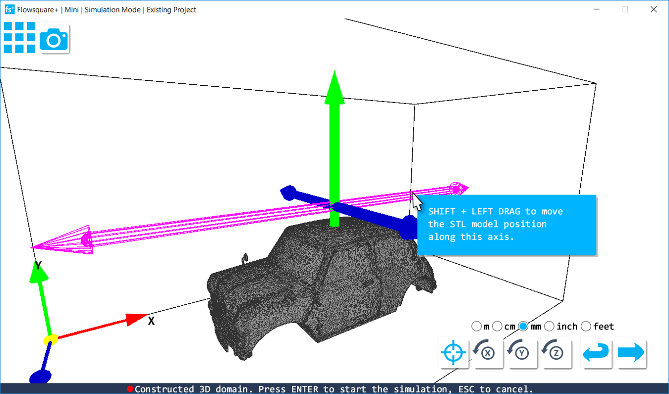
A constant wall temperature (K) of the wall specified by STL model (bc.stl). Setting 0, the wall is treated as adiabatic wall. Effective when cmode=1 (thermo fluid simulation mode). *The unit is (K; Kelvin). - unitSTL [0][2019R1 or later]
Unit of length used in the STL file (bc.stl). An option is chosen from radio buttons. This parameter option can also be chosen in the STL model loader. For more information see this page.- m
- cm
- mm
- inches
- feet
- xOffstSTL [0.0][2019R1 or later]
An offset distance (m) of the STL model in X-direction. This parameter can also be set in the STL model loader. For more information see this page. - yOffstSTL [0.0][2019R1 or later]
An offset distance (m) of the STL model in Y-direction. This parameter can also be set in the STL model loader. For more information see this page. - zOffstSTL [0.0][2019R1 or later]
An offset distance (m) of the STL model in Z-direction. This parameter can also be set in the STL model loader. For more information see this page. - normVecDirSTL [0][2019R1 or later]
Direction of normal vectors from STL model polygon. An option is chosen from radio buttons. The normal vectors point outwards in general STL files, and the default setting in Flowsquare+ follows that convention.- outwards
- inwards
- coordSTL [0][2019R1 or later]
Coordinate of STL polygons. Usually, they are constructed in right-hand coordinate in most CAD softwares.- Right-hand coordinate
- Left-hand coordinate
- xRotSTL [0.0][2019R1 or later]
An rotation angle (degrees) of the STL model around in X-axis. This parameter can also be set in the STL model loader. For more information see this page. - yRotSTL [0.0][2019R1 or later]
An rotation angle (degrees) of the STL model around in Y-axis. This parameter can also be set in the STL model loader. For more information see this page - zRotSTL [0.0][2019R1 or later]
An rotation angle (degrees) of the STL model around in Z-axis. This parameter can also be set in the STL model loader. For more information see this page - openPresFlag [0][2019R1 or later]
Pressure treatment of outflow boundary. An option is chosen from radio buttons. Normally, 0: Neumann condition is used, but for some case of (quasi-)closed configuration with local open boundary, 1: Dirichlet condition may be used.- Neumann condition
- Dirichlet condition (=presW).
- presAdjustFlag [1][2019R1 or later]
Enabling pressure adjustment such that the mean pressure equals presW. If openPresFlag=1 is used, presAdjustFlag is automatically set to be 0.- Disable
- Enable
- mu [1.0e-5]
Dynamic viscosity of fluid (Pa*s). Flowsquare+ assumes a constant viscosity. For standard condition, mu of the air is approximately 1.8E-5 (Pa*s). mu of the water is approximately 1.0E-3 (Pa*s). - Pr [0.7]
Prandtl number of the fluid. Usually, it takes approximately 0.7. Effective when cmode=1 (thermo-fluid simulation mode). - Sc [1.0][2018R2 or later]
Schmidt number of the fluid. Usually, it takes approximately 1. This value is effective when the mass fraction transport equation is also computed during simulation, by setting non-zero value for the boundary parameters in above, massfr# (# is a wildcard character for a color). - Cs [0.17][2018R2 or later]
Smagorinsky constant used in a Smagorinsky model for under-resolved turbulent motions. Usually, it takes 0.17. - ScT [0.7][2018R2 or later]
Turbulent Schmidt number used in a turbulent scalar flux model for under-resolved turbulent mixing effect. Usually, it takes 0.7. This value is effective when temperature and mass fraction transport equations are considered. - nfig [1000]
Frequency of saving snapshot images of simulation window. By setting nfig>0, snapshot images are saved in ./figs/ in the project directory once in every nfig time steps. The image file name begins with its time step. Saving images too frequently may affect computational speed negatively. - nfile [1000]
Frequency of saving instantaneous dump files of the simulation. By setting nfile>0, dump files are saved in ./dump/ in the project directory once in every nfile time steps. The dump files consist of u-velocity (ufld), v-velocity (vfld), w-velocity (wfld), pressure (pfld), and Y (yfld). Temperature (tfld) and density (rfld) are saved for cmode=1 (thermo-fluid simulation mode). Dump files at restart time step are necessary to restart the simulation. Saving dump files too frequently may affect computational speed negatively. - ndiv [4]
Interval mesh points of visualization objects such as velocity vectors, tracer particles, streamlines. These objects are (initially) generated at intervals of ndiv. - gfx [0.0]
External force in X-direction (m/s2). This value is effective when cmode=1 (thermo-fluid simulation mode). - gfy [0.0]
External force in Y-direction (m/s2). Usually, for gravity gfy=-9.8 (m/s2). This value is effective when cmode=1 (thermo-fluid simulation mode). - refMoment [0][2023R2.0 or later]
The reference point considered during fluid moment calculation.- Center of gravity of the object (assuming constant density)
- Geometric center of the object (mid-point of each direction)
- presRelax[1.0]
Relaxation parameter for pressure evolution. Usually 1.0 (0.0 ≤ presRelax ≤ 1.0). Set a lower velue if there is unphysical pressure oscillation inside the domain. - wfilWallBC [0.25][2020R1.0 or later]
Filter weight (0.0 <= wfilWallBC <= 1.0) for wall boundary construction. Using a higher value makes the constructed wall boundary smoother, but less accurate respect to the bitmap images the boundary was constructed with. peridir [0][no longer used in 2020R1.0 or later]
Direction to apply periodic boundary condition. An option is chosen from radio buttons.- No periodicity
- Periodicity in X-direction
- Periodicity in Y-direction
- Periodicity in Z-direction