The Easiest Computational Fluid Dynamics Software
 JP
JP
Flow simulation in a fishbowl
This page describes the procedure using newer version of Flowsquare+ 2023R1.0 or later.
1. Introduction
In this tutorial, we will perform a flow simulation in a container (goldfishbowl) with smooth curved surfaces, which can be achieved by using the subtraction function. All input files required to run the simulations presented can be downloaded below.
Input files
A typical computational time of this case is approximately 10 minutes per 1000 time steps with a typical Core i7 PC with the parallelism setting, parallel = 3, in parameter setting.
2. Simulation domain
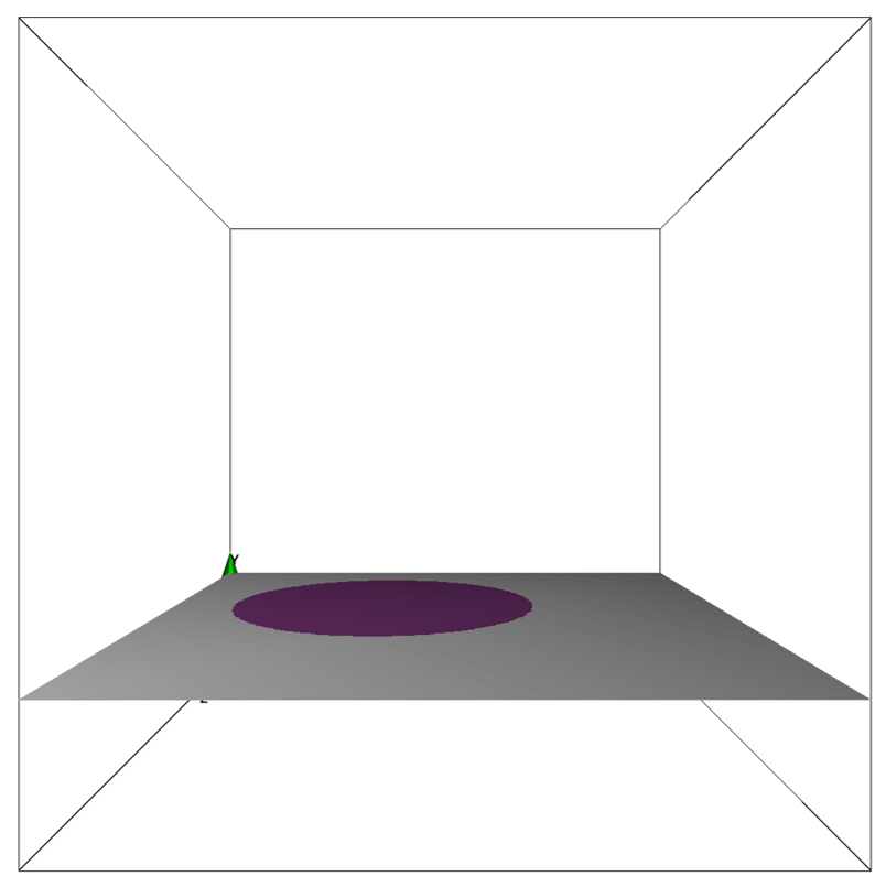
The most important part of any simulation is to clearly define what is simulated. In this tutorial, we will perform a flow simulation in a fishbowl filled with water, with a pump that generate water flow as the following schematic.
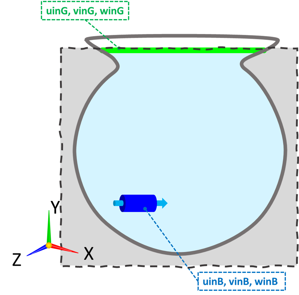
Here, the blue object is a pump that produces water flow in the x-direction, and the gray (dark and light) indicates the wall boundary. The water level in the fishbowl is denoted by the green line. The dotted line indicates the simulation domain. As in "Flow through the Bottom and Keel of a Yacht", this time we use a simplified representation of the water surface boundary condition, which is slip wall boundary condition with zero velocity in out-of-plane direction of the water surface.
3. 3D model construction
General rule of constructing 3D boundary conditions is explained in here. It is recommended to constcut each elemental object one by one repeatedly. For example, first create and check the fishbowl, then create and check the pump, then create and check the slip wall boundary condition, and so on, repeating the creation and checking of each element part.
In this simulation, the following boundary condition colors are used for the fishbowl.
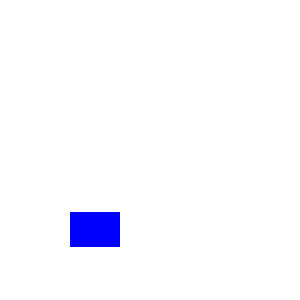
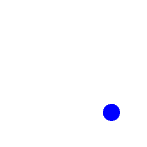
Preset colors- ■ Pump suction and discharge port
- ■ Slip wall boundary for the simplified representation of the water surface (zero velocity only in the y-direction, the out-of-plane direction of the water surface)
- ■ fishbowl (since we're using the subtraction tool, ■ represents the fluid region of the fishbowl)
- ■ Solid wall
The selection of these boundary condition colors is a gradual process of creation and confirmation for each element part, and not all color schemes are determined from the beginning.
The paint image pixel sizes are irrelevant to the actual physical domain dimensions. However, it is a good idea to use more or less similar aspect ratio between the bitmap images and the domain dimensions. In the present cases, 1 pixel of the bitmap images corresponds to 1mm in the physical space.
The figures below show the bitmap image for boundary construction and the orientation of each image within the simulation domain.

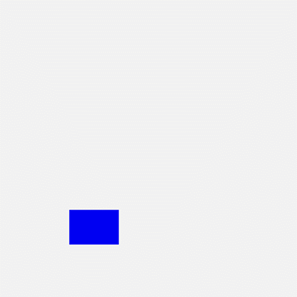
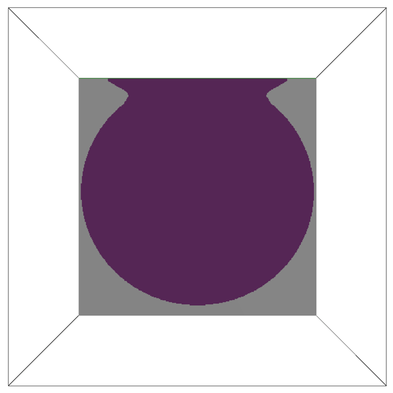
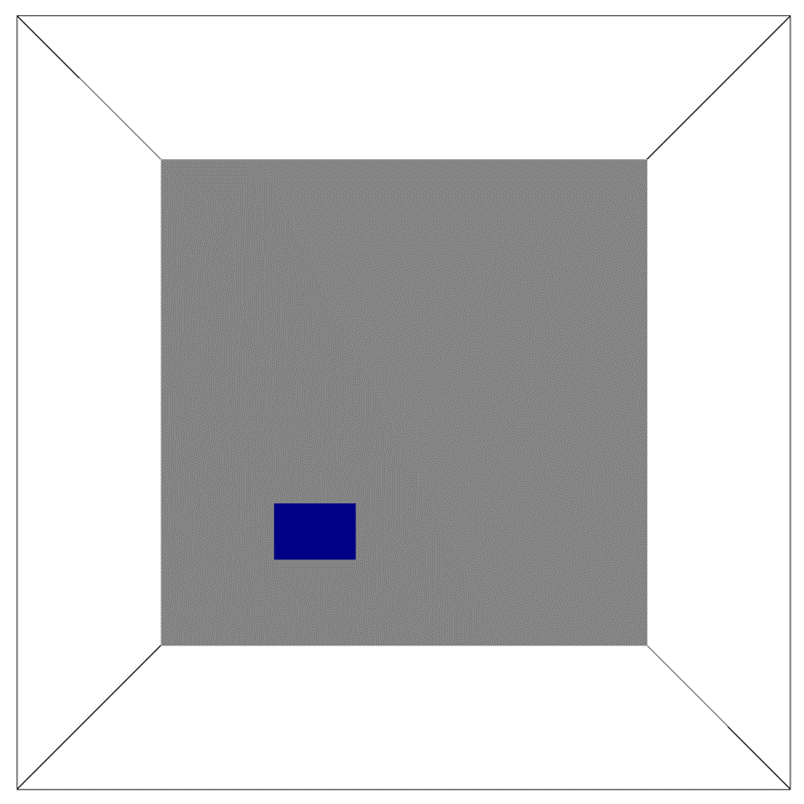

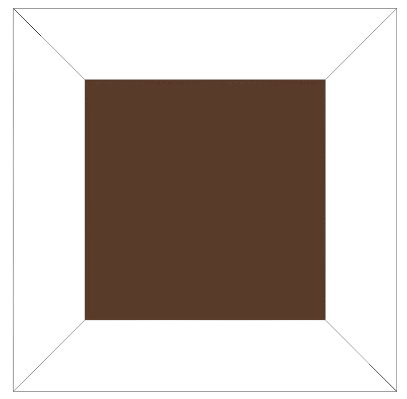


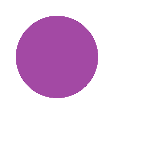
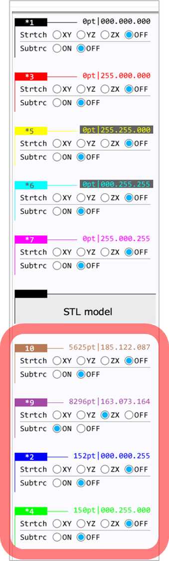
Here, first for the sfishbowl, we apply the stretching tool in the ZX direction for the object specified by the non-preset color ■ (click here to see how to select the tool). In this way, the ZX cross sectional shape (bcZX0.bmp) is stretched along both the XY cross sectional (bcXY0.bmp) and YZ cross sectional (bcYZ0.bmp) shapes shown above to construct a fishbowl consisting of smooth 3D surfaces.
To construct the fish bowl, the model shape of the non-preset color ■ needs to be subtracted from the model shape of the non-preset color ■. This can be achieved by setting the subtraction tool (Subtrc) and the order of boundary construction appropriately as shown in the below image.
The above procedure for applying the construction tools and changing construction order is summarized in the below figures. These selections are saved in input/bmp.txt, which is automatically generated under the project directory. Once they are set, they do not need to be set again for the same project.
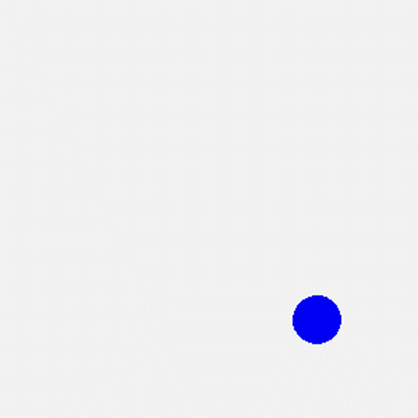
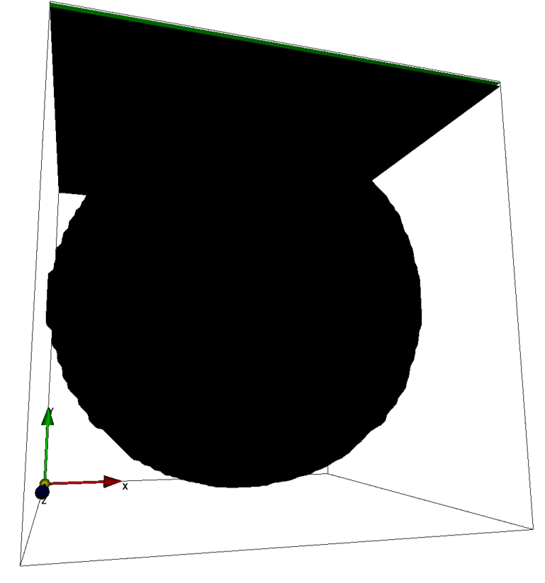
The final 3D model constructed by the above procedure is shown below. The outside of the fishbowl is defined as the back side of the 3D model because it is all solid area, and reflections are not taken into account and it is just black. However, as shown in the animation on the right, the inside of the fishbowl is a fluid region, defined as the front side of the 3D model, and light reflection is correctly taken into account. Thus, we can see that we have correctly constructed the fishbowl. In the animation, you can also see the pump constructed in the preset blue color inside the fishbowl.
4. Input parameters
Below explains several important aspects of the present simulation example. General description of parameters in Flowsquare+ are explained here.
- cmode
Taken as 0 for the fluid simulation mode (constant temperature and density). - lx, ly, lz
The domain dimensions are (lx, ly, lz) = (0.3, 0.3, 0.3) m. - nx, ny, nz
The number of mesh points needs be determined based on the required spatial resolution. Here, we will use (nx, ny, nz) = (75, 75, 75). - rhoW
Taken as the water density of 997.0 kg/m^3. - uinB, vinB, winB
The fluid velicity driven by the pump is 1m/s in the x-direction. Therefore, uinB=1.0 m/s. The defalt values of vinB and winB are zero, so they do not need to be set in the parameter. - uinG, vinG, winG
For the simplified representation of the water surface boundary condition, we use the slip wall boundary condition with zero velocity in out-of-plane direction (Y-direction) of the water surface. Therefore, (uinG, vinG, winG) = (-,0,-) m/s. - mu
The viscosity of water is 1.0E-3 (kg/m/s).
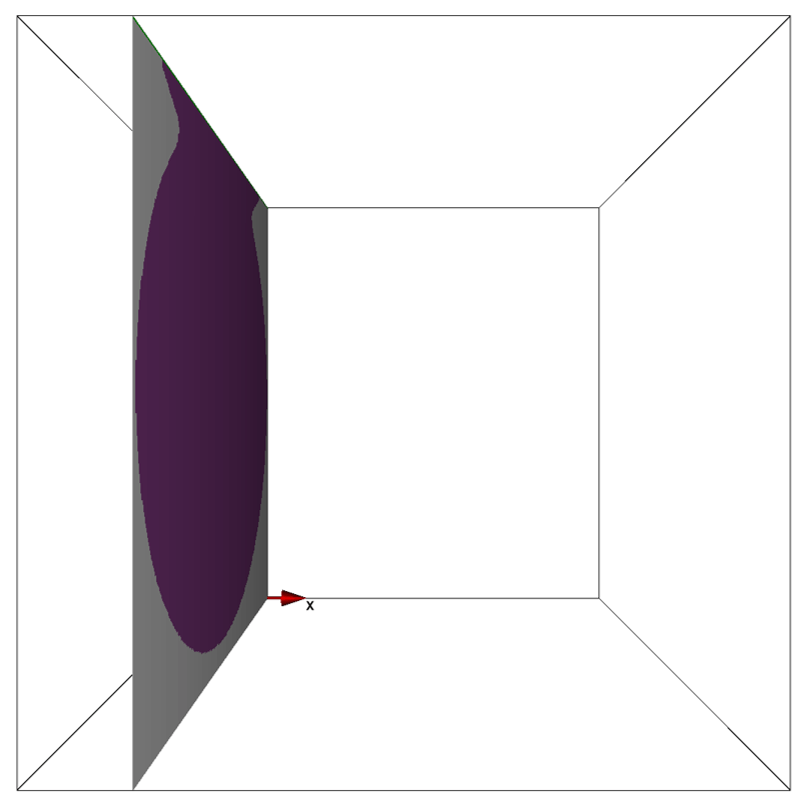
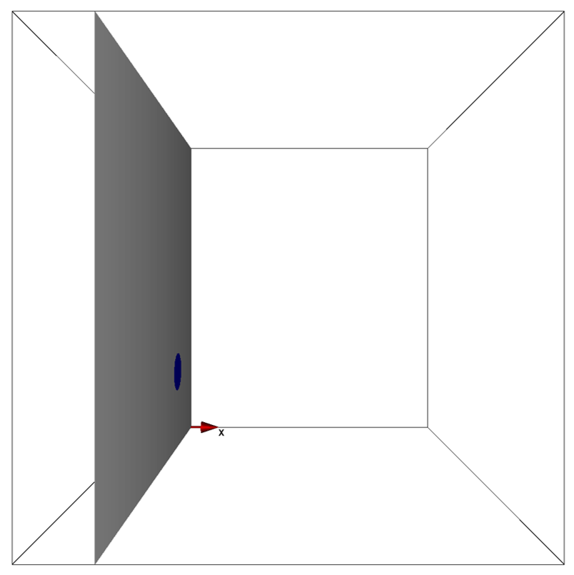
5. Simulation results
The simulation result data saved by Flowsquare+ is visualized with Paraview (a free external visualization software) as shown in the below figure. (click here to see how to visualize the Flowsquare+ data with Paraview).
The inverse tool was used in this simulation example to construct a container shape composed of three-dimensional smooth surfaces. In the case of a rectangular container such as a usual aquarium, the model can be constructed without using the inverse tool, by simply using five walls with two-dimensional planes.