The Easiest Computational Fluid Dynamics Software
 JP
JP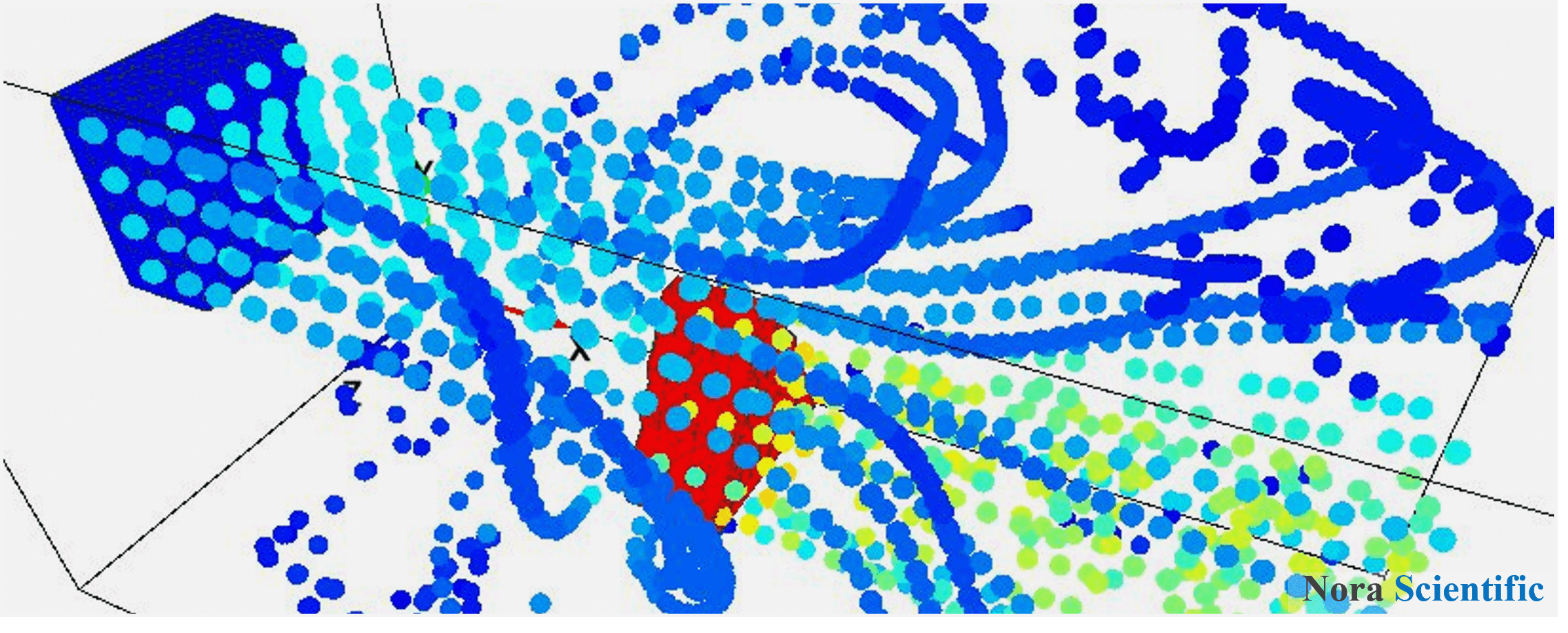
Demonstration for tracer particle function
* A bug fix for the tracer particle function has been implemented in version 2023R2.2. Please use version 2023R2.2 or later if there is no special reason.
1. Introduction
This tutorial describes the use of tracer particles to help understand fluid simulation results. All input files required to run the simulations presented can be downloaded below.
Input files
This simulation requires a computation time of about 1 minute for 1000 steps on an Intel COREi7 laptop with parallel level parallel=3, in parameter setting.
2. Simulation domain
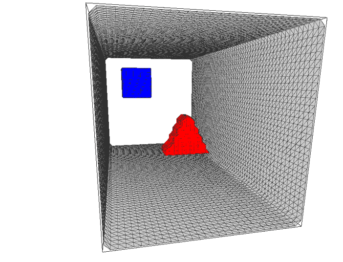
In this simulation, we consider a domain in which there are two "pumps" that generate water flow in a channel surrounded on all sides by walls. The flow field is visualized by tracer particles flowing out of these two pumps.
3. 3D Model Construction
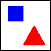
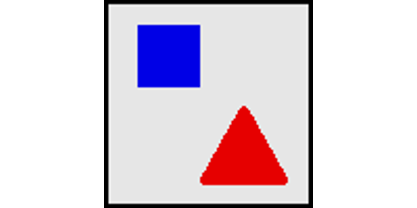
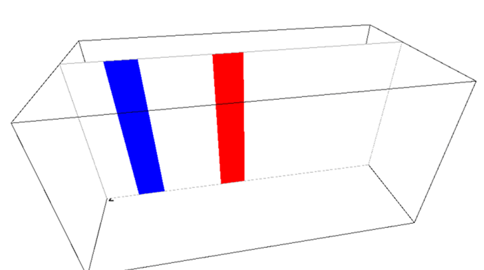
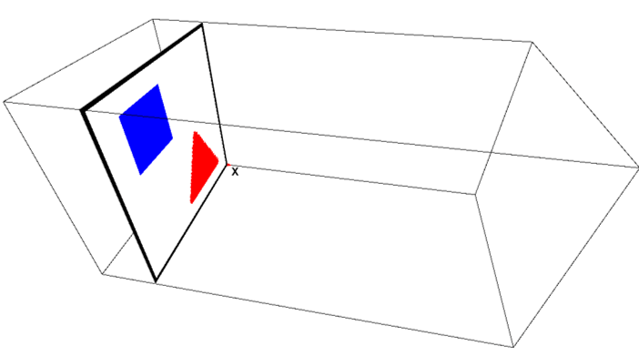
Please refer to here for the basic rules for creating a 3D model. The boundary conditions handled in this simulation example all consist of "(a) model with a uniform 2D cross-section" or "(b) model constructed by third angle projection". In this simulation example, we consider a pump defined by a blue inflow boundary condition with a square shape and a pump defined by a red inflow boundary condition with a triangular shape, as follows. The wall boundary, specified in black, defines the walls of the channel. The figures below show the orientation of the bitmap image for the boundary condition and the constructed boundary condition within the simulation domain.
4. Input parameters
The following is a description of parameters of particular importance in this simulation. For a description of general calculation parameters, please click here.
- cmode
Taken as 0 for the fluid simulation mode (constant temperature and density). - lx, ly, lz
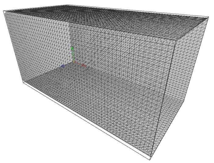
x-, y-, and z-directional domain sizes of 10 m, 5 m, and 5 m, respectively. - nx, ny, nz
The number of mesh points needs be determined based on the required spatial resolution. Here, we will use (nx, ny, nz) = (60, 30, 30). - rhoW
Specify 1.2 kg/m^3, the density of air. - uinB, vinB, winB
The flow velocity from the blue pump is 10 m/s in the positive x direction; therefore, uinB = 10.0 m/s. The default values for vinB and winB are zero and need not be specified. - uinR, vinR, winR
The flow velocity from the red pump is 20 m/s in the positive x direction; therefore, uinR = 20.0 m/s. The default values for vinR and winR are zero, so there is no need to specify them. - mu
Specify 2.0E-5 (kg/m/s) as the viscosity coefficient of air. - ndiv
Specify ndiv=2 as the size and display interval of the visualization object, scaled by 2 grid points.
5. Running simulation and results
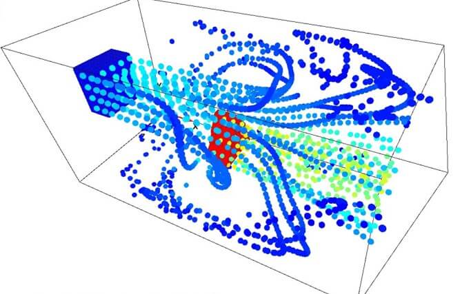
After starting the simulation, select "Tracer Particles"  from the "Tool Pane". In the blue and red pump regions, you can see the particles being generated and flow out at intervals of ndiv set by the parameters. The following movie was created from a series of images output every 10 time steps.
The density of fed particle are determined based on ndiv in the simulation parameters.
Generally, the default setting should be fine, but various parameters for tracer particles can be specified in the viz-related parameters. Maximum number of particles can be set by numTracerParticles in the viz-related parameters. The particle feed interval and its velocity factor are set by particleFeedInterval and particleVelocityMultiple, respectively. The relative size of the particles can be specified by particleSize. Tracer particles are only generated under blue or red inflow boundary conditions. They are not generated in inflow boundary regions of other colors.
You can also color particles with a color map based on the currently displayed physical quantity. This allows for an easy understanding of the evolution of the physical quantity at the location of each particle. For coloring, select "colouring visualization object based on the current physical quantity" in the "Tool Pane".