The Easiest Computational Fluid Dynamics Software
 JP
JP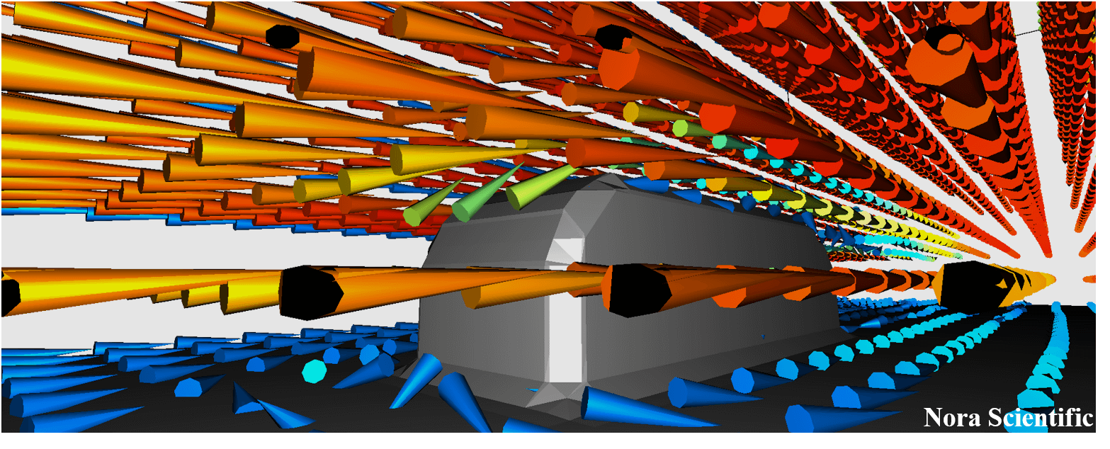
Flowsquare+ Wind Tunnel (Modified Model)
1. Introduction
In this tutorial, we will modify the original wind tunnel case to perform a simlation with a different model. Input files required for this simulation is downloaded below.
Input files
A typical computational time of this case is approximately 3 minutes per 1000 time steps with a typical Core i7 PC with the maximum parallelism setting (parallel in parameter setting).
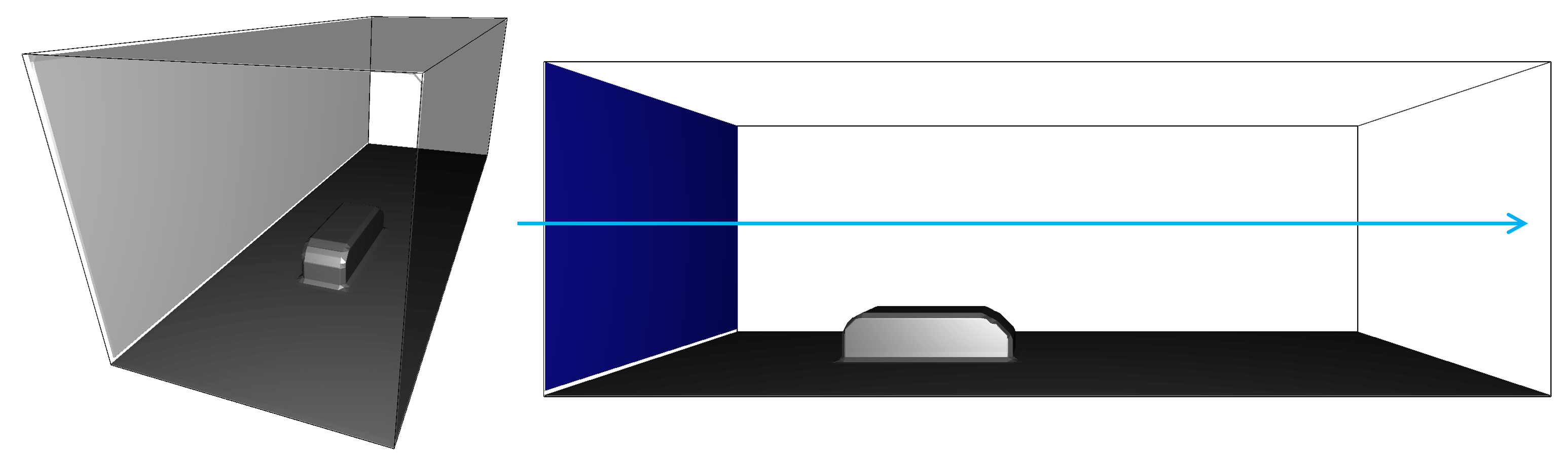
2. Domain Configuration
The domain configuration is shown in below, which is similar to what we saw in this wind tunnel tutorial, but instead of airfoid we will place a lump.
A typical computational time of this case is approximately 3 minutes per 1000 time steps with a typical Core i7 PC with the maximum parallelism setting (parallel = 3 in parameter setting).
3. Construction of Boundary Condition
General rule of constructing 3D boundary conditions is explained in here.
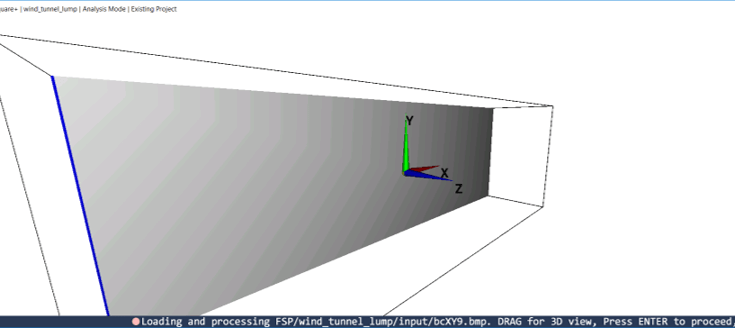
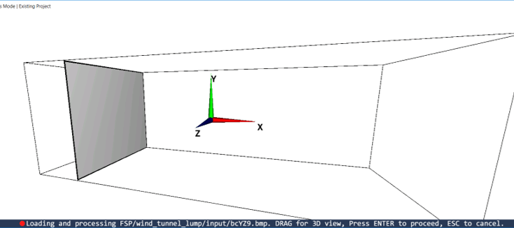
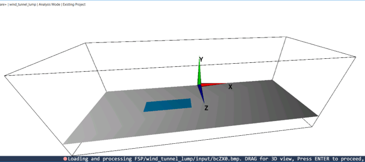
In this simulation, we will specify (1) wind tunnel walls with preset BLACK color, (2) an inflow boundary condition with preset BLUE color, and (3) the lump object and floor with NON-preset colors, magenta and light blue. Each of these parts is constructed using the rules of "(a) Model with a uniform 2D cross-section" and "(b) Model constructed by third angle projection".
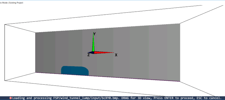
In the this simulation, instead of making boundary configuration images from scratch, we modify the input paint images for the original wind tunnel case. More specifically, we modify bcXY0.bmp and add bcZX0.bmp to realize a simulation of a lump object in the same wind tunnel (you do not need to modify paint images for the wind tunnel, bcXY9.bmp and bcYZ9.bmp).
Likewise, you can find an example simulation case, and modify the input files to perform a simulation you actually want to run!


4. Numerical Parameters
- cmode
cmode is taken as 0 for the fluid simulation mode (constant density, constant temperature, single phase for gas and liquid flows).
- lx
The domain length in X-direction is 3m.
- ly
The domain length in Y-direction is 1m.
- lz
The domain length in Z-direction is 1m.
- nx、ny、nz
The number of mesh points needs be determined based on the required spatial resolution. Here, we will use (nx, ny, nz) = (120, 40, 40), which are different from the original wind tunnel case. This is because in this case, the test object (lump) has relatively thick compared to the airfoil, and having less ny still reasonably resolve the most of fluid motions around the object.
- rhoW
Fluid density is taken as 1.2 kg/m^3, which corresponds to the air property at a standard condition.
- uinB
Inflow velocity at the blue inflow boundary is taken as 20.0 m/s.
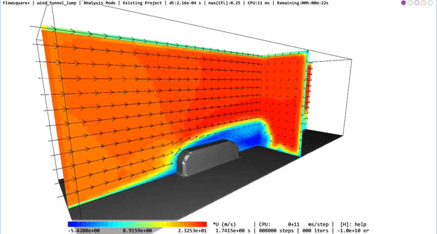
5. Performing Simulation
Using the input files provided in the above link, you can perform the simulation with following steps. You can also perform various vizualization and analysis in-situ or post, including calculating forces imposed on the object (see tool pane).