The Easiest Computational Fluid Dynamics Software
 JP
JP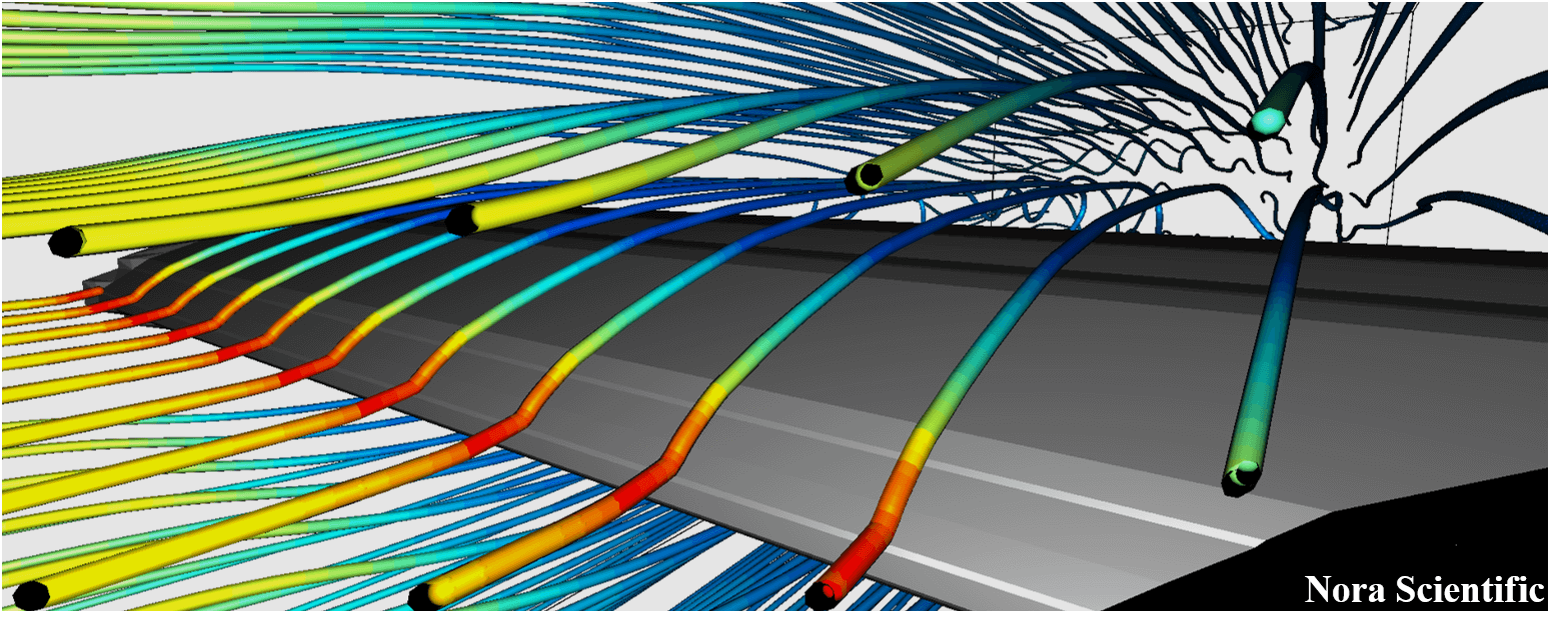
Flowsquare+ Wind Tunnel
1. Introduction
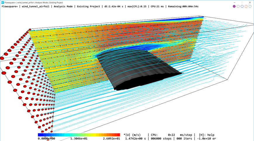
Using Flowsquare+, you can computationally perform wind tunnel experiments on your PC. This tutorial explains how to set up an airfoil in your wind tunnel to visualize flows and calculate various hydrodynamic forces (lift, drag, etc...).
All the required input files for this test case can be downloaded below.
Input files
A typical computational time of this case is approximately 3 minutes per 1000 time steps with a typical Core i7 PC with the maximum parallelism setting (parallel in parameter setting).
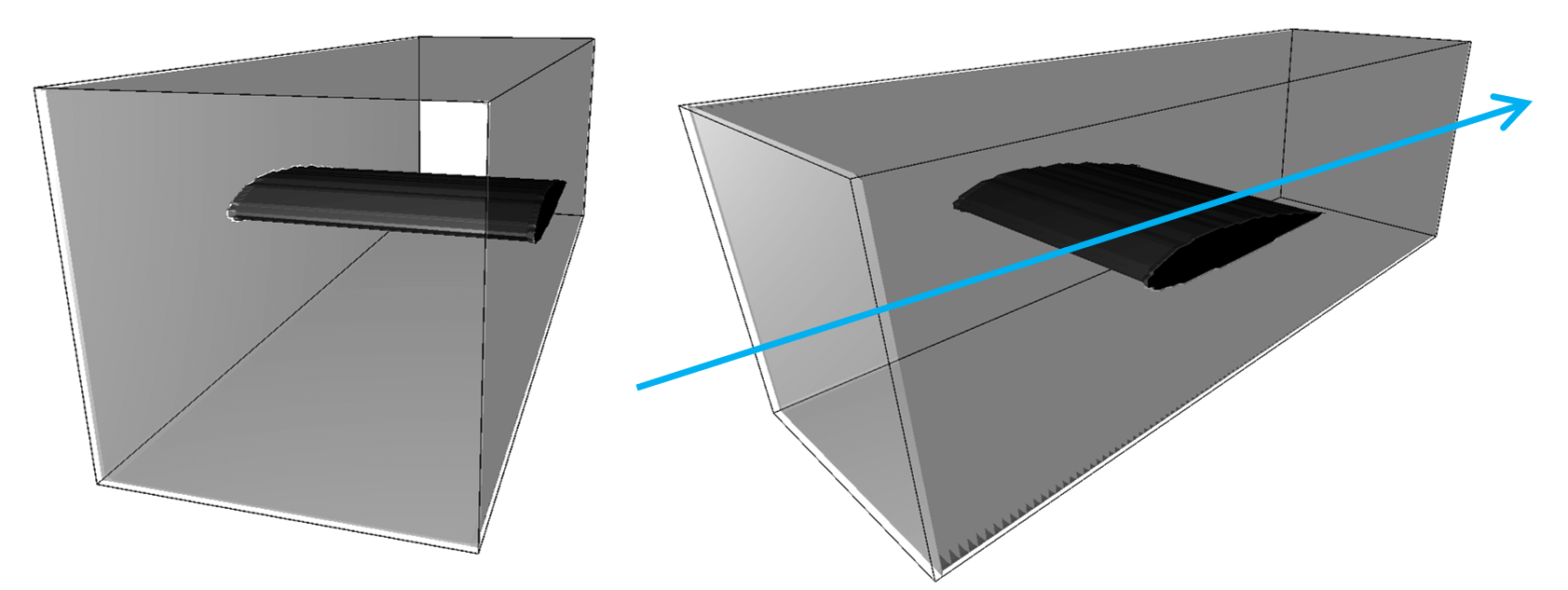
2. Domain Configuration
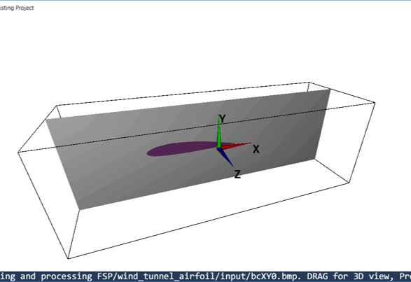
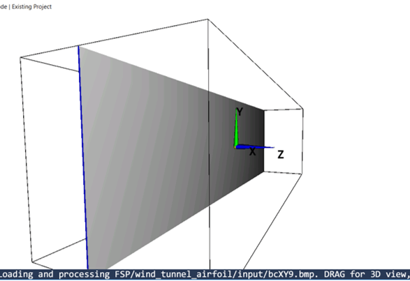
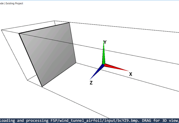
Our virtual wind tunnel looks something like below images. Walls are situated on four sides, and there is an inflow boundary on the left and an outflow boundary on the right along the X-direction.
You do not need to use any preset boundary configuration for this case (as all input files are prepared for you), but using it could reduce paint images you need to prepare.
3. Constructing Boundary Conditions
General rule of constructing 3D boundary conditions is explained in here.
In this simulation, we will specify (1) wind tunnel walls with preset BLACK color, (2) an inflow boundary condition with preset BLUE color, and (3) the airfoil with NON-preset color. Each of these parts is constructed using the rule of "(a) Model with a uniform 2D cross-section".
The paint image pixel sizes can be irrelevant to actual physical domain dimensions. However, it is a good habit to use more or less similar aspect ratio between images and domain dimensions. For example, you can set a rule on your own that 1m length corresponds to 800 pixels in the paint images.


4. Computational Parameters
Several important parameters are explained here. More thorough information about parameters can be found here.
- cmode
cmode is taken as 0 for the fluid simulation mode (constant density, constant temperature, single phase for gas and liquid flows).
- lx
The domain length in X-direction is 3m.
- ly
The domain length in Y-direction is 1m.
- lz
The domain length in Z-direction is 1m.
- nx、ny、nz
The number of mesh points needs be determined based on the required spatial resolution. Here, we will use (nx, ny, nz) = (80, 80, 40), which yields different mesh size for each direction. This is because (1) the velocity change in X- and Y-directions is expected to be much greater than that in Z-direction, and (2) The thickness of airfoil is relatively thin, requiring a little better resolution to resolve the object in Y-direction.
You may change the number of mesh points to see how different spatial resolution influences the solution.
- rhoW
Fluid density is taken as 1.2 kg/m^3, which corresponds to the air property at a standard condition.
- uinB
Inflow velocity at the blue inflow boundary is taken as 20.0 m/s.
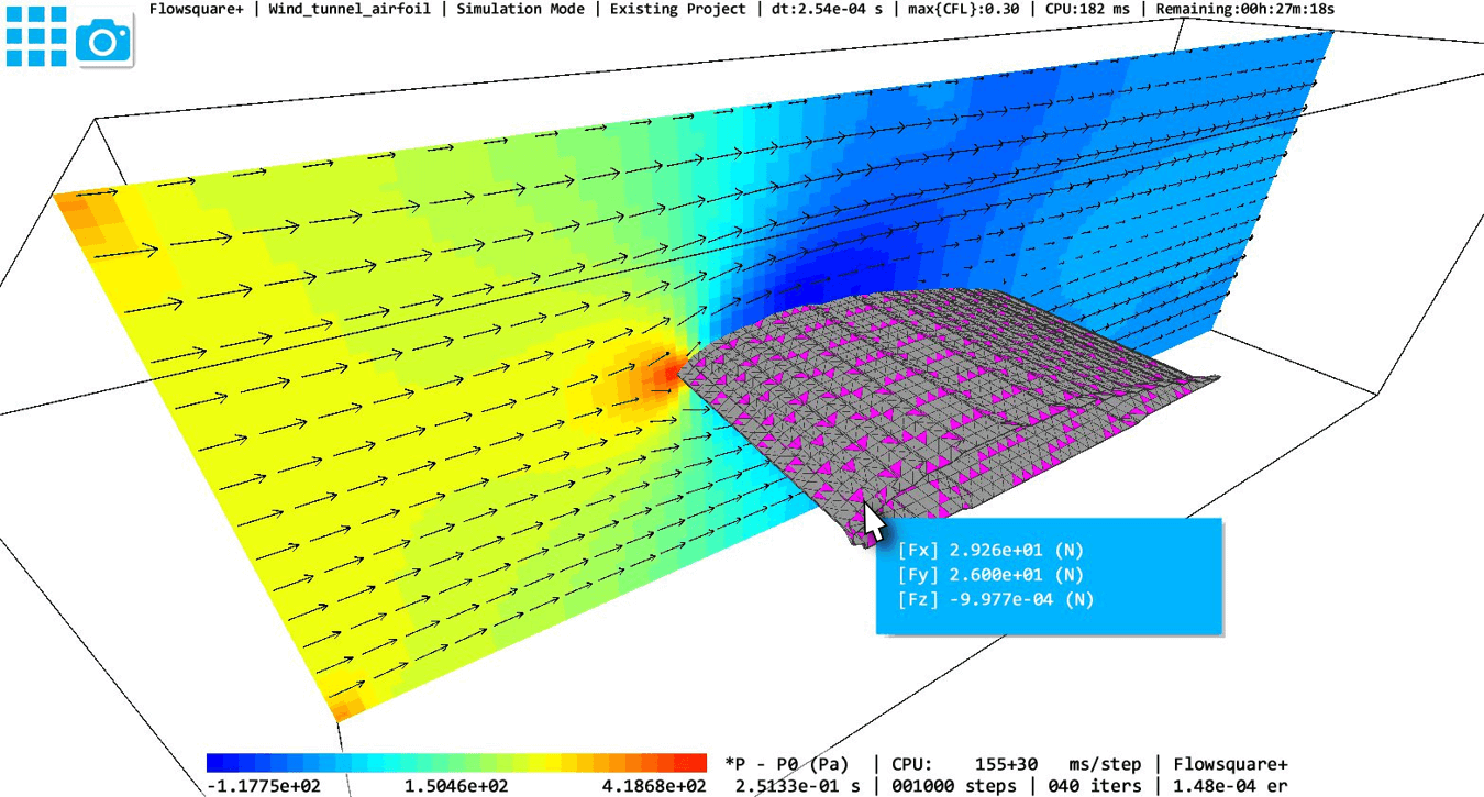
5. Performing Simulation and Analysis
Using the input files provided in the above link, you can perform the simulation with following steps. To compute hydrodynamic forces imposed on the airfoil, you can use  from the tool pane.