The Easiest Computational Fluid Dynamics Software
 JP
JP
A Simulation with an STL Model
1. Introduction
The present simulation is based on the case we already used in "Getting Started with Flowsquare+", but with few modifications, to get to know more about Flowsquare+.
All the required input files for this test case can be downloaded below.
Introduction
A typical computational time of this case is approximately 5 seconds per 1000 time steps with a typical Core i7 PC with the maximum parallelism setting (parallel in parameter setting).
2. Domain configuration
The present case is very similar to the example case we have already used in "Getting Started with Flowsquare+", except that
- The present case is for thermofluid simulation with temperature variations, and
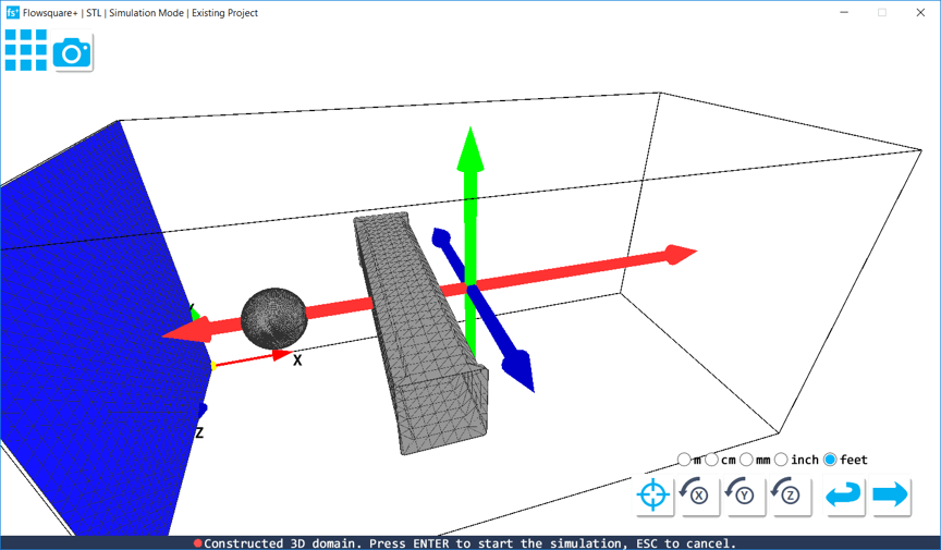
- A CAD model (a spherical object) is additionally used for an additional boundary condition.
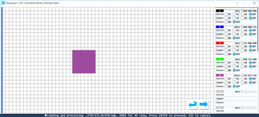
Following figures show the boundary configuration image (bcXY0.bmp) and the CAD model (bc.stl).
3. Simulation Parameters
Several important parameters are explained here. More thorough information about parameters can be found here.
- cmode
cmode is taken as 1 for the 1:Thermo fluid simulation mode (varying temperature ideal-gas flows).
- uinB
X-direction velocity component for the blue inflow boundary is taken as 10.0 m/s.
- tempW
Initial fluid temperature is taken as 300K.
- tempB, temWall
The temperature for the blue inflow boundary and wall boundary specified by non-preset colors are an adiabatic condition.
- tempWallSTL
The temperature of the wall specificed by the CAD model is 400K.
- unitSTL, xOffstSTL, yOffstSTL, zOffstSTL
The unit and position of the CAD model can be adjusted graphically in STL model loader.
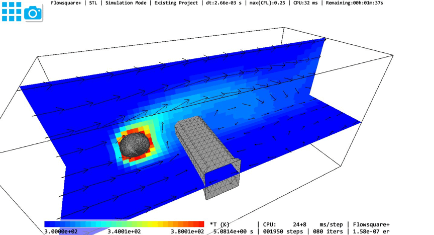
4. Simulation results
The following figure shows an instantaneous temperature field. You can also change the position of the CAD model and perform simulations to see the effect of the spherical object on the solution!