The Easiest Computational Fluid Dynamics Software
 JP
JP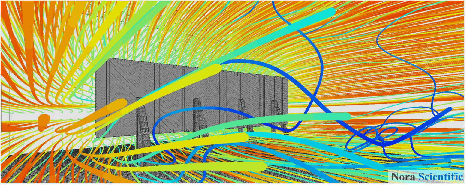
Estimation of a Drag Force on a Signborad
1. Introduction
Here, we will simulate a flow field around a signboard, and through some analysis, we would like to obtain insights into usefulness and limitation of the popular estimation method of hydrodynamic drag forces based on the drag coefficient.
The drag coefficient \(C_D\) is often used to estimate the drag force \(F_D~\rm{(N)}\) as
\begin{equation} F_D=C_D \frac{\rho u^2}{2}A. \:\:\:\:\:\:\:\:\:\:\:\:\rm{Eq. (1)} \end{equation}Here, \(\rho~\rm{(kg/m^3)}\) is the fluid density (constant), \(u~\rm{(m/s)}\) is the fluid (mean) velocity, and \(A~\rm{(m^2)}\) is the projection area of the object respect to the flow direction.
The drag coefficient of the plate placed perpendicular to the stream-wise direction depends on the aspect ratio of the plate. If the dimensions of the plate are \(a\times b~\rm{(m^2)} (a > b)\),
- \(a/b\sim1\) ⇒ \(C_D\approx1.1\)
- \(a/b\sim4\) ⇒ \(C_D\approx1.2\)
- \(a/b\sim10\) ⇒ \(C_D\approx1.3\)
- \(a/b\sim20\) ⇒ \(C_D\approx1.4\).
It should be noted that these values are obtained under Reynolds numbers where \(C_D\) shows almost constant variation. Also, in these experimental setups, the plate is located far away from other physical boundaries, to minimize the effect of these boundaries on the drag force.
In this page, we construct a model signboard by using bitmap images, and perfrom simulations around it, to obtain the drag force. For a comparison, we also construct a model of a plate placed perpendicular to the flow, which is not affected by another physical boundary (mimicing the experiental setup for \(C_D\)). Also, we compare obtained drag forces with the one estimated by using Eq. (1).
All the required input files for this test case can be downloaded below.
(A) Signboard model
(B) Plate model (a plate placed perpendicular to the flow, which is not affected by another physical boundary)
The computational time of this case is approximately 10 minutes per 1000 time steps with a typical Core i7 PC with the maximum parallelism setting (parallel = 4 in parameter setting).
2. Model construction
(A) Signboard model
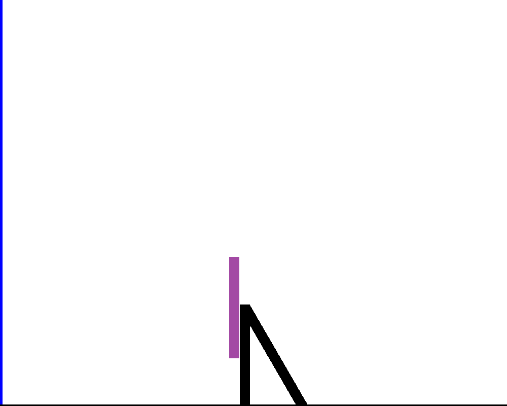
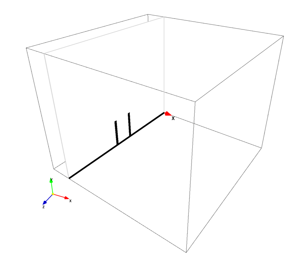
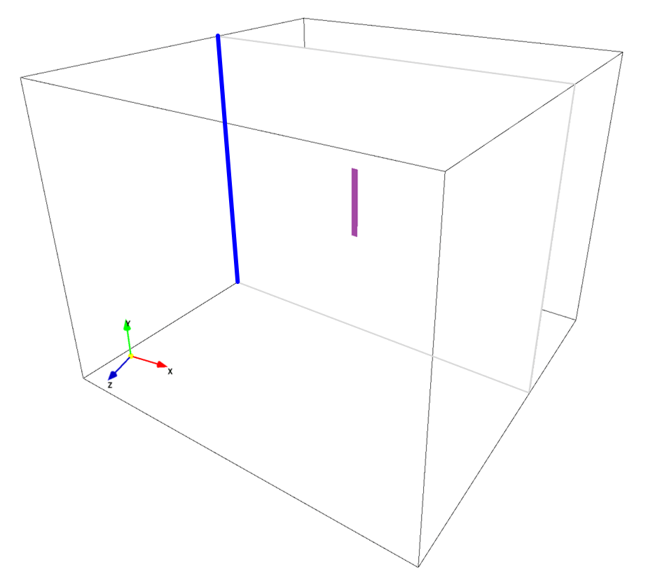
General rules of constructing 3D boundary conditions using paint images are explained in here. In the present simulation, following three bitmap images are used to construct the model signboard. The three colors used in the paint images, and parts these colors specify are:
- Wall boundary: signboard, non-preset color, purple
- Wall boundary: pillar and ground, preset color, black
- Inflow boundary: preset, blue
In the present simulation, the signboard body is specified by a non-preset color(s), while other wall boundaries are specified by preset color, so that we can compute a drag force acting on the signboard body alone. For this purpose, we can also construct the signboard body with a preset color (black) and the pillar and ground using a non-preset color(s).
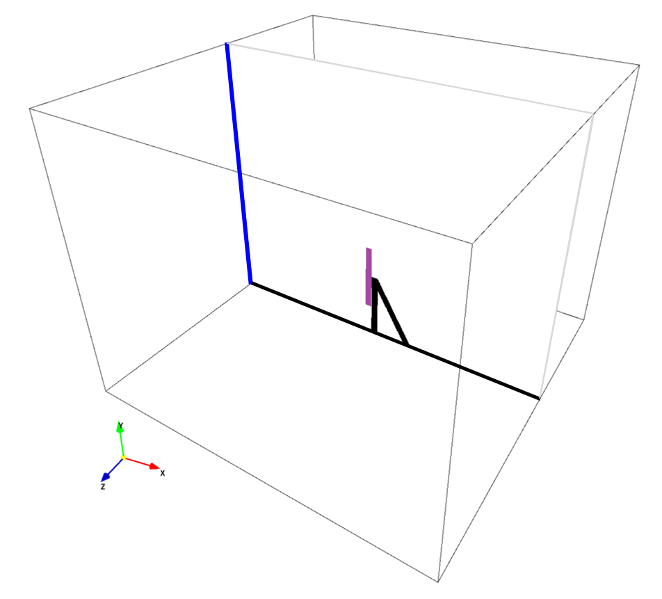
The pixel size of each bitmap image does not neet to be proportional to the physical domain dimensions. The domain dimensions are set as \(L_x, L_y, L_z\) specified in the parameter editor, and all bitmap images are extended/compressed by interpolation before after they are loaded. However, it is recommended that bitmap images reflect the physical domain dimensions. In the above simulation files, all images are created for 2 pixels per 1cm physical length. The signboard body pixel dimensions are specified by 400 pixels \(\times\) 200 pixels in bcYZ0.bmp, and the signboard area is \(A=2\times1~\rm{(m^2)}\).
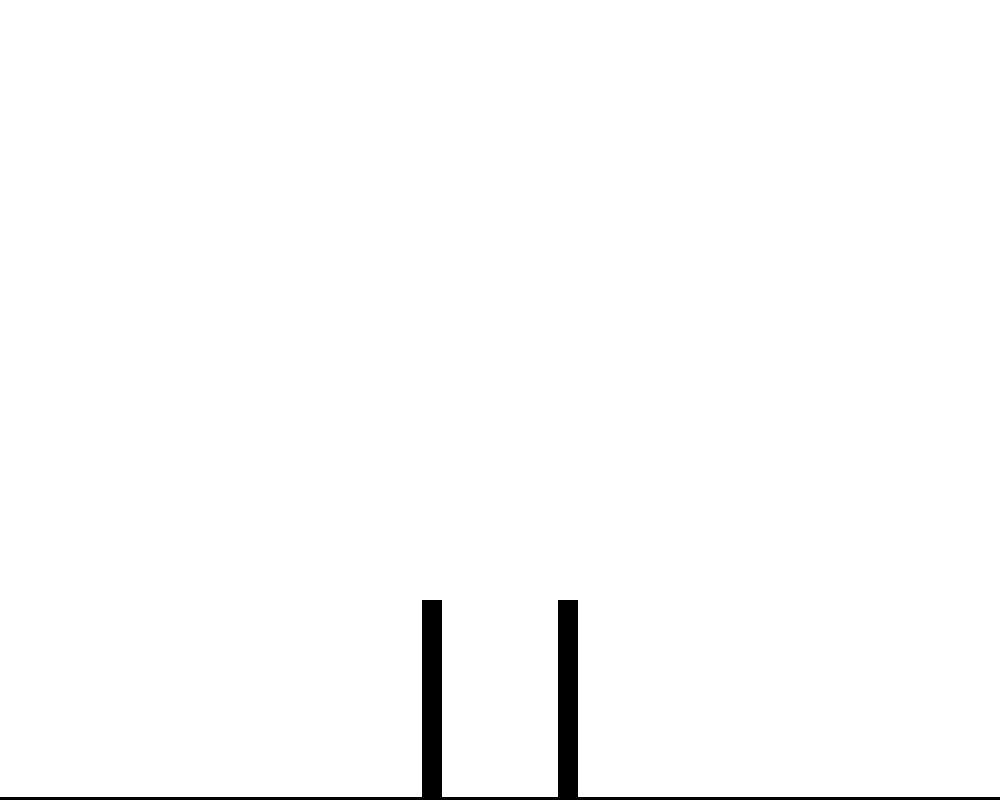
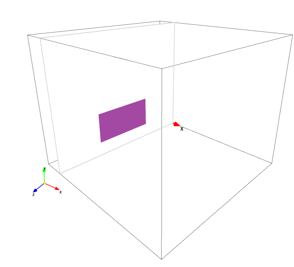
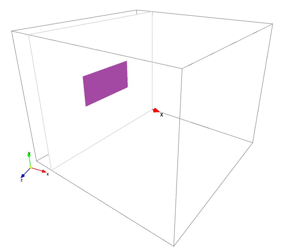
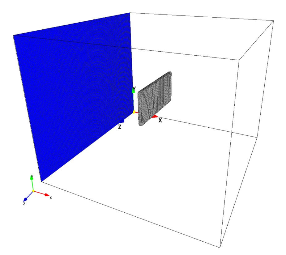
(B) Plate model
The plate model is just a plate normal to stream-wise direction located middle of the simulation domain without a pillar or a ground. It is specified by two bitmap images. The size and dimensions of plate are the same as the signboard body (\(A=2\times1~\rm{(m^2)}\)).
3. Numerical parameters
Several important parameters are explained here. The same parameter set is used for (A) Signboard model and (B) Plate model. More thorough information about parameters can be found here.
- cmode
cmode is taken as 0 for the 0:Fluid simulation mode (constant temperature flows). - lx
The domain length in X-direction is 5m. - ly
The domain length in Y-direction is 4m. - lz
The domain length in Z-direction is 5m. - nx、ny、nz
(nx, ny, nz) = (400, 80, 100) - uinW
Initial x-component fluid velocity is taken as 10m/s. The other components (vinW, winW) are zero (=default value), so they do not need to be specified. - vinB
The inflow velocity from the blue boundary is taken as 10m/s. The other components (vinB, winB) are zero (=default value), so they do not need to be specified.
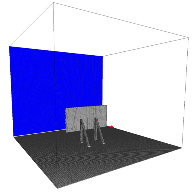
4. Simulations and post-analysis, discussion
Let's start the simulation. You can visualize the flow field during and/or after the simulation (using the analysis mode). You need to run the simulation long enough so that initial effect (artifact) disappears from the simulation domain and the solution reaches quasi-steady state. To make sure this, you can place a measurement probe downstream during the simulation.
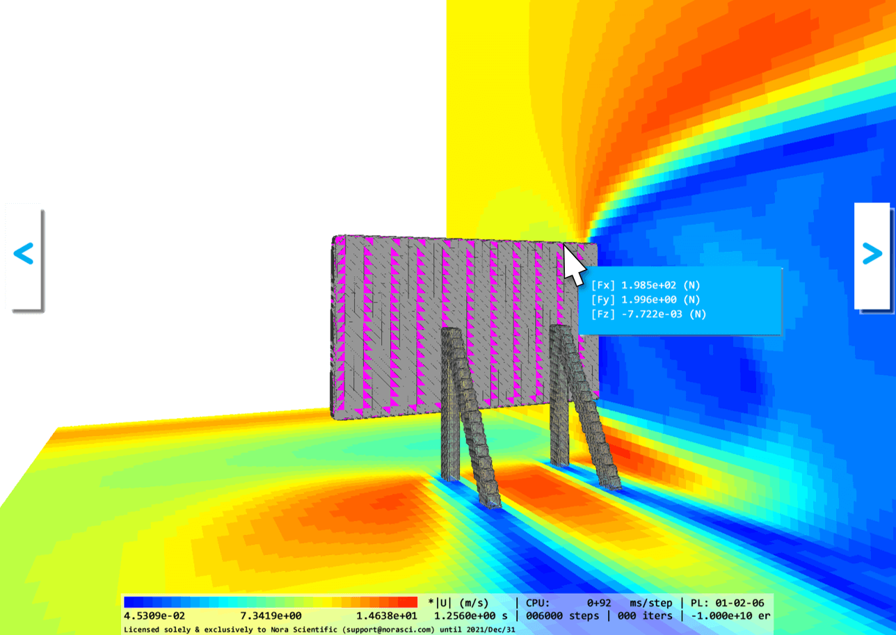
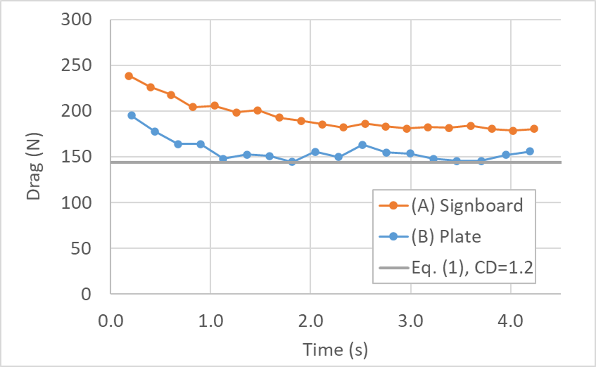
By using  found in the tool pane, you can compute the forces acting on the signboard body and plate. Also, based on the simulation conditions, \(\rho=1.2~\rm{(kg/m^3)}\), \(u=10~\rm{(m/s)}\), \(A=2~\rm{(m^2)}\) and \(C_D=1.2\), Eq. (1) estimates the drag force to be \(144~\rm{(N)}\). The below figures are comparison of these values.
Since this is unsteady simulation (i.e. not Reynolds averaged Navier-Stokes simulation), right after the initialization (\(t=0\)), the computed forces are much higher than the one obtained from Eq. (1), each of which converges around a certain value later times. After \(t=1-2~\rm{(s)}\), the solution seems to reach quasi-steady state, and the force for (B) Plate model transitions around the value estimated by Eq. (1). However, the force for (A) Signboard model shows 20-30% higher values.
When it comes to the drag force of perpendicular plate, we tends to use \(C_D=1.2\) without further consideration. However, as the present simulations showed, this drag coefficient is based on the configuration where the other physical boundaries (surrounding walls, etc..) have small effect on the object of interest. If these walls are located relatively close to the object of interest (like the signboard and the ground), the drag coefficient tends to be greater.