The Easiest Computational Fluid Dynamics Software
 JP
JP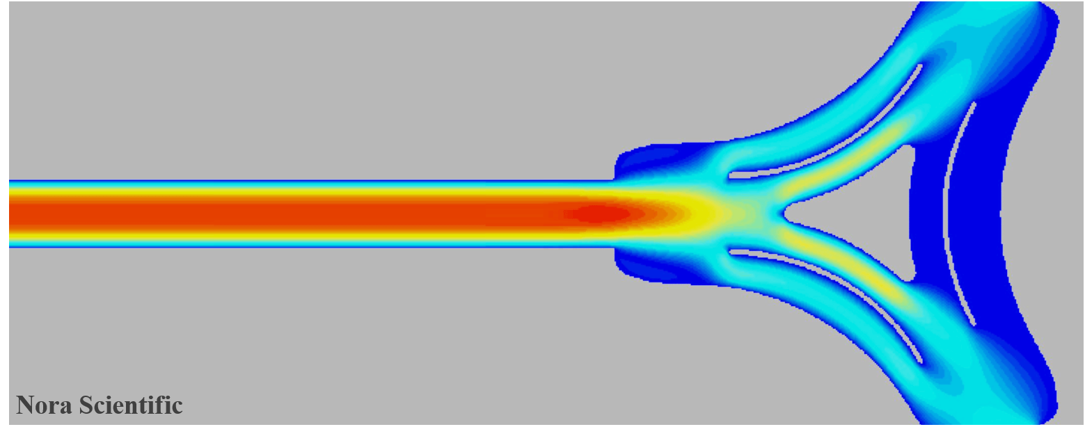
Flow Splitter
1. Introduction
Many fluid flows around us can be represented by 2-dimensional flows, in which case, we can predict the flow with 2D CFD with much less computational costs.
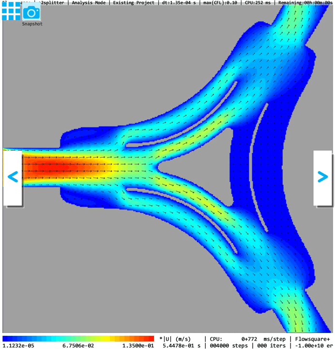
This tutorial simulates such a flow in the "flow splitter", often used in medical and chemical fields.
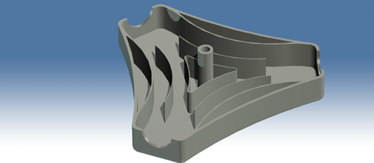
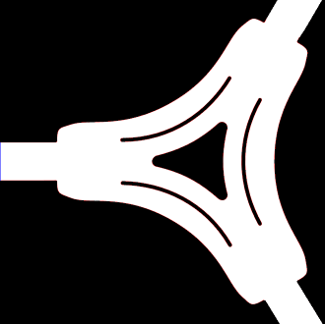
The present model flow splitter is based on the one publically available at GRABCAD, and the paint image (bcXY0.bmp) to be used for boundary construction is constructed based on the downloadable CAD file.
All the required input files for this test case can be downloaded below.
Input files
A typical computational time of this case is approximately 1 minute per 1000 time steps with a typical Core i7 PC with the maximum parallelism setting (parallel in parameter setting). Evolution of computational time is shown in a below figure.
2. Simulation parameters
Several important parameters are explained here. More thorough information about parameters can be found here.
- cmode
cmode is taken as 0 for the fluid simulation mode (constant density, constant temperature, single phase for gas and liquid flows).
- lx
The domain length in X-direction is 0.07m (7cm).
- ly
The domain length in Y-direction is 0.07m (7cm).
- nx、ny、nz
The number of mesh points needs be determined based on the required spatial resolution. Here, we will use (nx, ny, nz) = (384, 384, 1), which yields the same mesh size for each direction.
You may change the number of mesh points to see how different spatial resolution influences the solution.
- rhoW
Fluid density is taken as 1.2 kg/m^3, which corresponds to the air property at a standard condition.
- uinB
Inflow velocity at the blue inflow boundary is taken as 0.1 m/s (10 cm/s).
3. Performing simulation
Using the input files provided in the above link, you can perform the simulation with following steps.
The below figure shows instantaneous fluid speed overlaid by velocity vectors, which was visualized after the simulation using the "analysis mode".