The Easiest Computational Fluid Dynamics Software
 JP
JP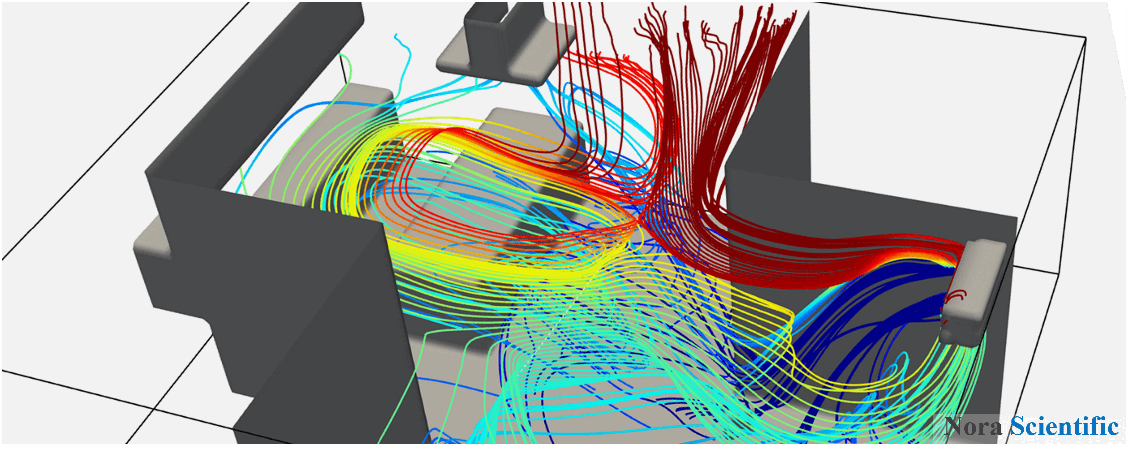
AC flow simulation based on a floor plan
1. Introduction
In this tutorial, we construct a 3D model based on an actual floor plan of a house, and perform AC-cooling thermo-fluid simulations with and without a circulation fan in Living, Dining and Kitchen area. All the input files required for the present three cases can be downloaded below.
A typical computational time of this case is approximately 3 minutes per 1000 time steps with a typical Core i7 PC with the parallelism setting, parallel = 3, in parameter setting
2. Simulation domain
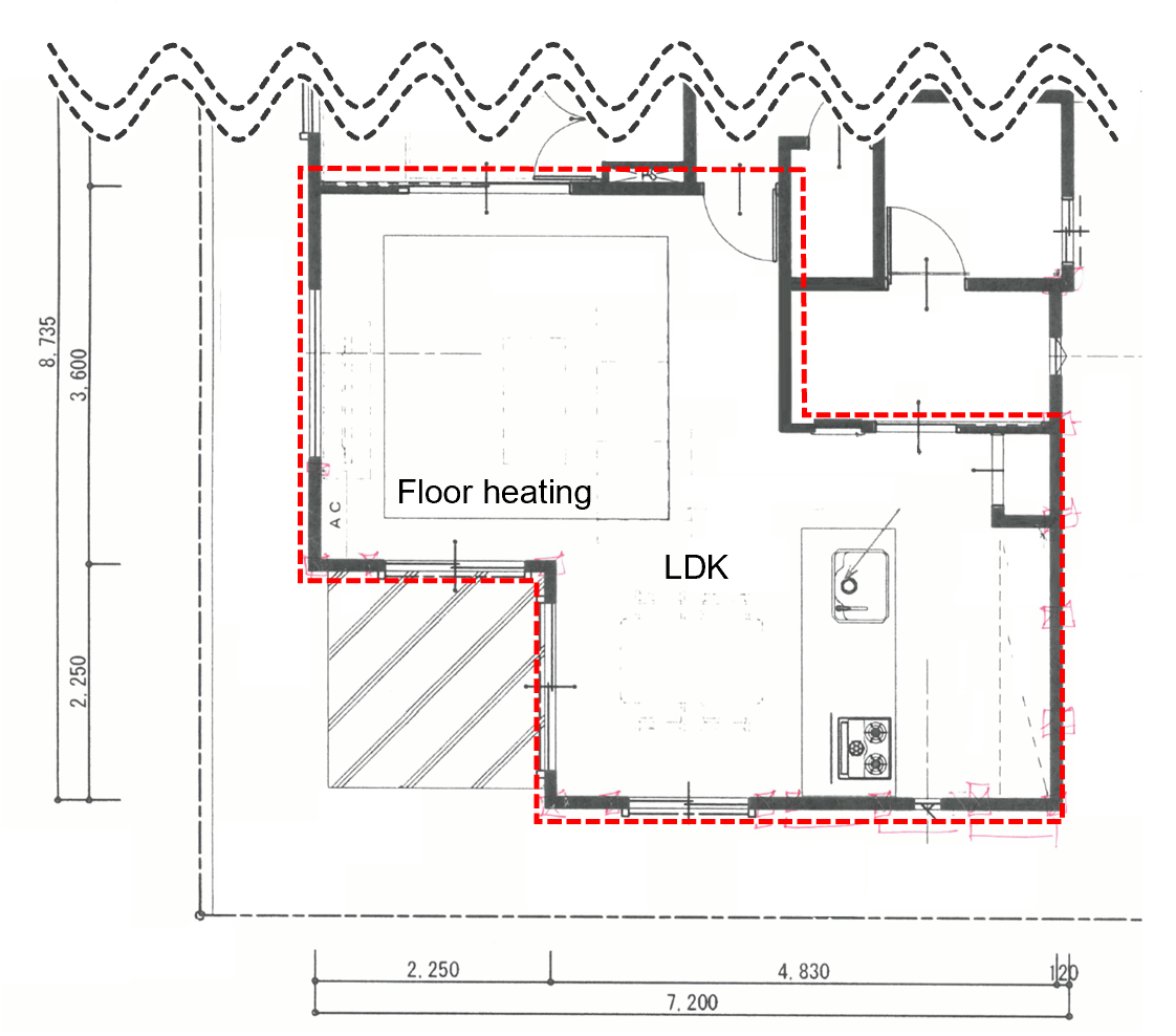
It is most important to clarify the target of simulation. In this tutorial, we simulate the air conditioning in the LDK area shown in the floor plan.
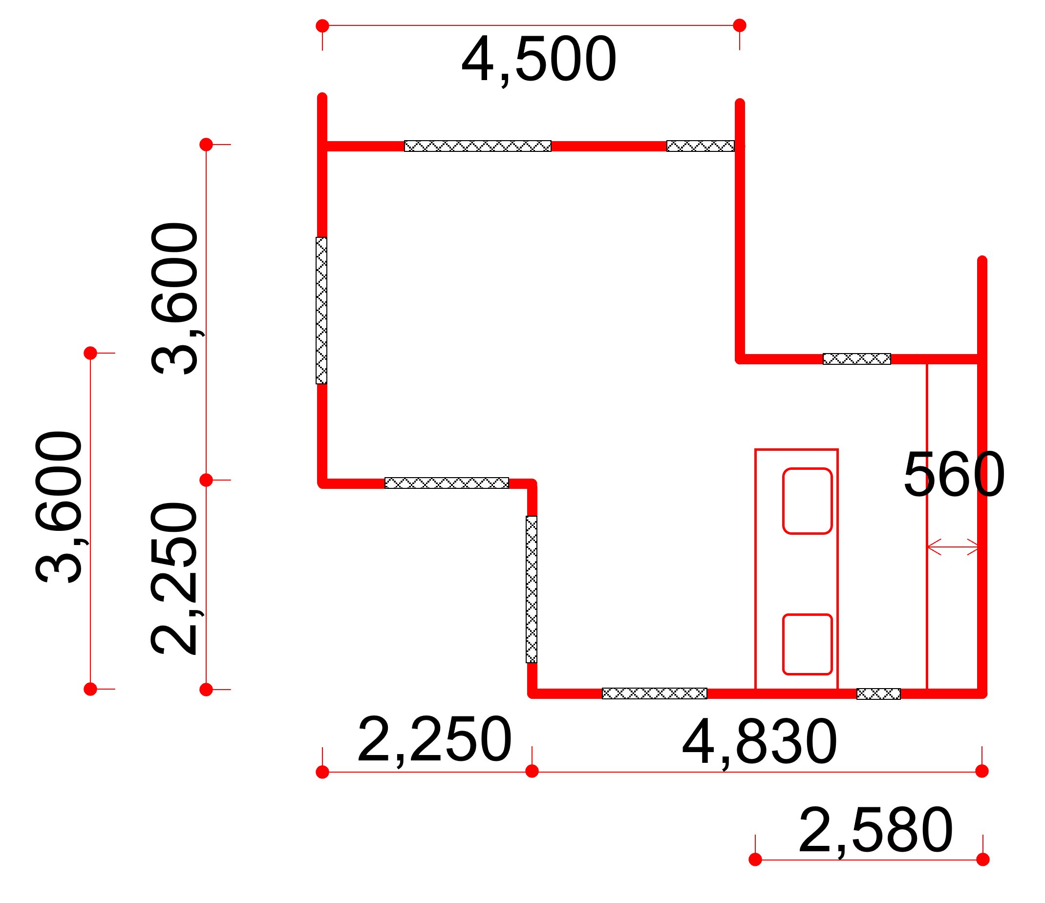
Below figure shows the actual floor plan of a house, and the LDK area is highlighted in red dashed line. The AC location is also shown in the bottom-left corner in the living area. The LDK area is not a simple rectangular shape. Therefore we perform this optimization so that single AC can cool the entire LDK area effectively.
To clarify the simulation domain setting more, we can trace the LDK shape in the above actual floor plan, and traced LDK schematic and dimensions are shown in the below figure. You can use a software such as Microsoft Powerpoint or Adobe Illustrator to trace the original floor plan. Here, information regarging height are:
- From floor to the ceiling: 2,500mm
- From floor to the kitchen surface: 900mm
- From floor to the kitchen counter surface: 900mm
- From kitchen counter surface to the bottom of kitchen cupboard: 700mm.
3. Construction of 3D model
General rule of constructing 3D boundary conditions is explained in here. It is recommended to constcut each elemental object one by one repeatedly. For example, first construct only the floor and check in 3D, then construct outer walls using another color and check in 3D, then construct the kitchen using another color and check in 3D, ..., until all the objects are constructed in different colors. Each elemental object is 3D object with 2D crosssectional shape, and construction is relatively straightforward.
To construct the 3D model, we use below colors to specify elemental objects in the model configuration bitmap images. However, the color choice is made one elemental object by one elemental object, and not something we can determine for all elemental objects at once beforehand.
Also, we used the preset colors, black and yellow, for the sidewall and ceiling, which could be also constructed by using non-preset colors like other objects. The choice of using the preset colors is because we may want to hide the sidewall and ceiling for visibility during visualization of the simulation results (objects constructed with non-preset colors are treated as one object, and cannot be displayed/non-displayed individually). Note that usually the preset yellow color is used for inflow boundaries. However, by setting all inflow velocity components to be zero, a boundary specificed by the yellow color (and other inflow related preset colors) is treated as wall condition.
- ■ Side wall
- ■ AC air exit
- ■ AC air intake
- ■ Circulation fan
(Combination case only) - ■ Ceiling
- ■ AC body
- ■ Non-fluid region
- ■ Kitchen counter
- ■ Kitchen cupboard and counter
- ■ Ventilation fan
(not functioning in the simulation) - ■ Floor
The paint image pixel sizes are irrelevant to the actual physical domain dimensions. However, it is a good habit to use more or less similar aspect ratio between the bitmap images and the domain dimensions. In the present cases, 1 pixel of the bitmap images corresponds to 1cm in the physical space. Therefore, since the horizontal length of the LDK space is 7080mm (2250-4830mm), the bitmap images have the horizontal length of 708 pixels (please see the above "Traced LDK area and dimensions").
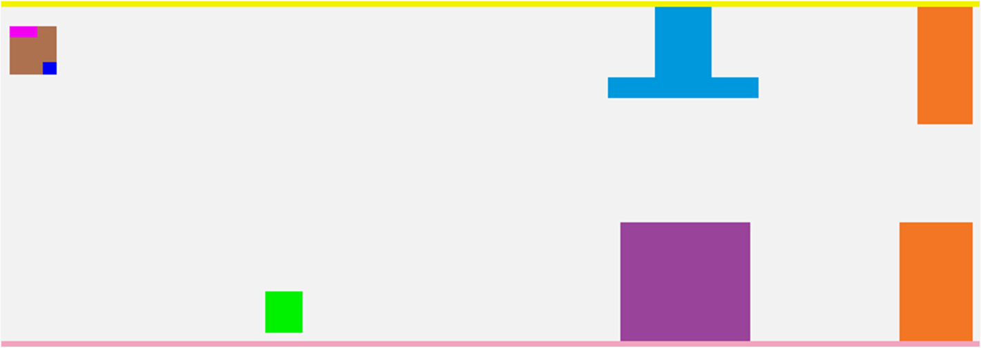

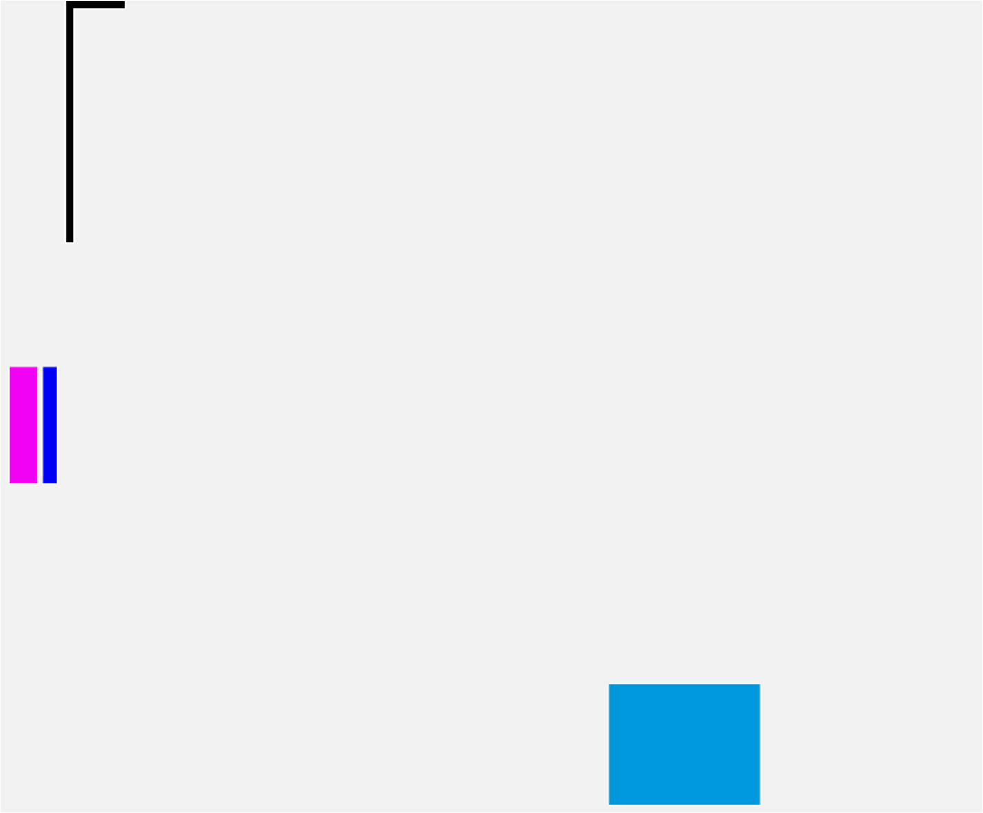
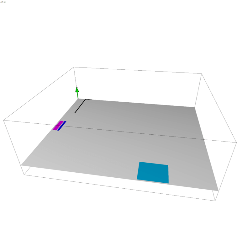
Above images show model configuration bitmap images used in the present simulation. The alignment of each bitmap image respect to the simulation domain is also shown. The difference between the reference and combination cases is the presence of the circulation fan specified by the preset green color.
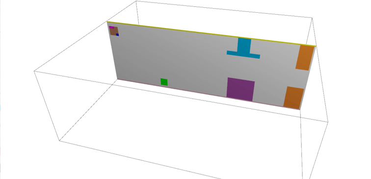
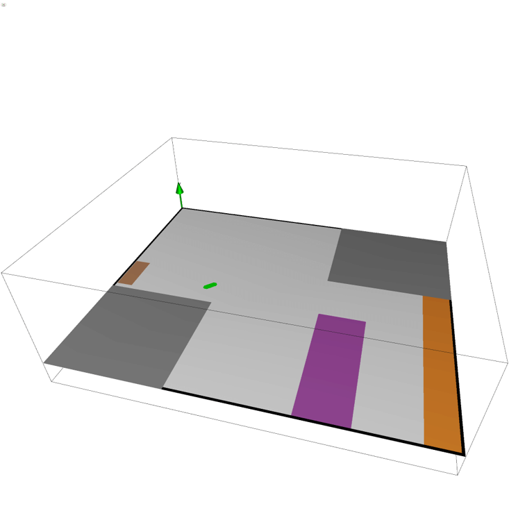
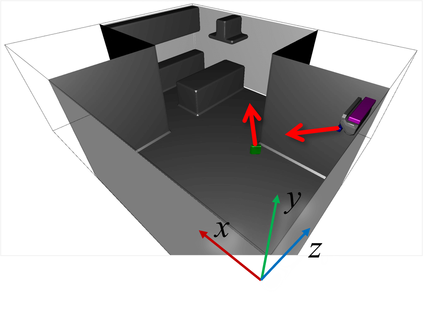
The constructed model (boundary condition) is shown below. The flow directions from the AC and the circulation fan are set as below, but they can be parametrized for optimization.
4. Input parameters
Several important parameters are explained below. More thorough information about parameters can be found here.
- cmode
Taken as 2 for the thermo-fluid simulation mode (varying temperature and density) - lx, ly, lz
The domain dimensions in x, y and z directions are 7.08, 2.50 and 5.85m, respectively. - nx, ny, nz
The number of mesh points in x, y and z directions are 140, 50 and 120, respectively. - tempW
Initial room air temperature is taken as 303 K. - uinB, vinB, winB
The flow speed from the AC exit is 1.4m/s, and 30 degree downwards towards x-direction. Therefore, uinB = 1.4*cos(30 deg) = 1.22 m/s, vinB=-1.4*sin(30 deg) = -0.707 m/s, and winB = 0. - tempB
The air temperature from the AC exit is set to be 293 K. - uinM, vinM, winM
The intake area of the AC is a half of that of exit. Therefore, intake fluid speed is approximately 0.7 m/s, and towards negative y-direction. Therefore, uinM = 0, vinM = -0.7 m/s, winM = 0. - tempM
The fluid temperature into the intake should not be constrained. Therefore specify "-" (hyphen) for tempM. - tempWallK, tempWall
The wall boundaries constructed by non-preset colors and preset black yield adiabatic condition. So set to be 0 (zero). - uinG, vinG, winG (for combination case)
The flow speed from the circulation fan is the same as AC exit flow speed, which is 1.4m/s and direction is (1,1,1). Therefore, uinG = vinG = winG = 0.81 m/s. - tempG(for combination case)
The fluid tempearture from the cirulation fan is the temperature of fluid flowing into the fan. Therefore, the fluid temperature should not be constrained, so it is set to be "-" (hyphen) for tempG. - gfy
Y-direction gravity is -9.8 m/s^2.
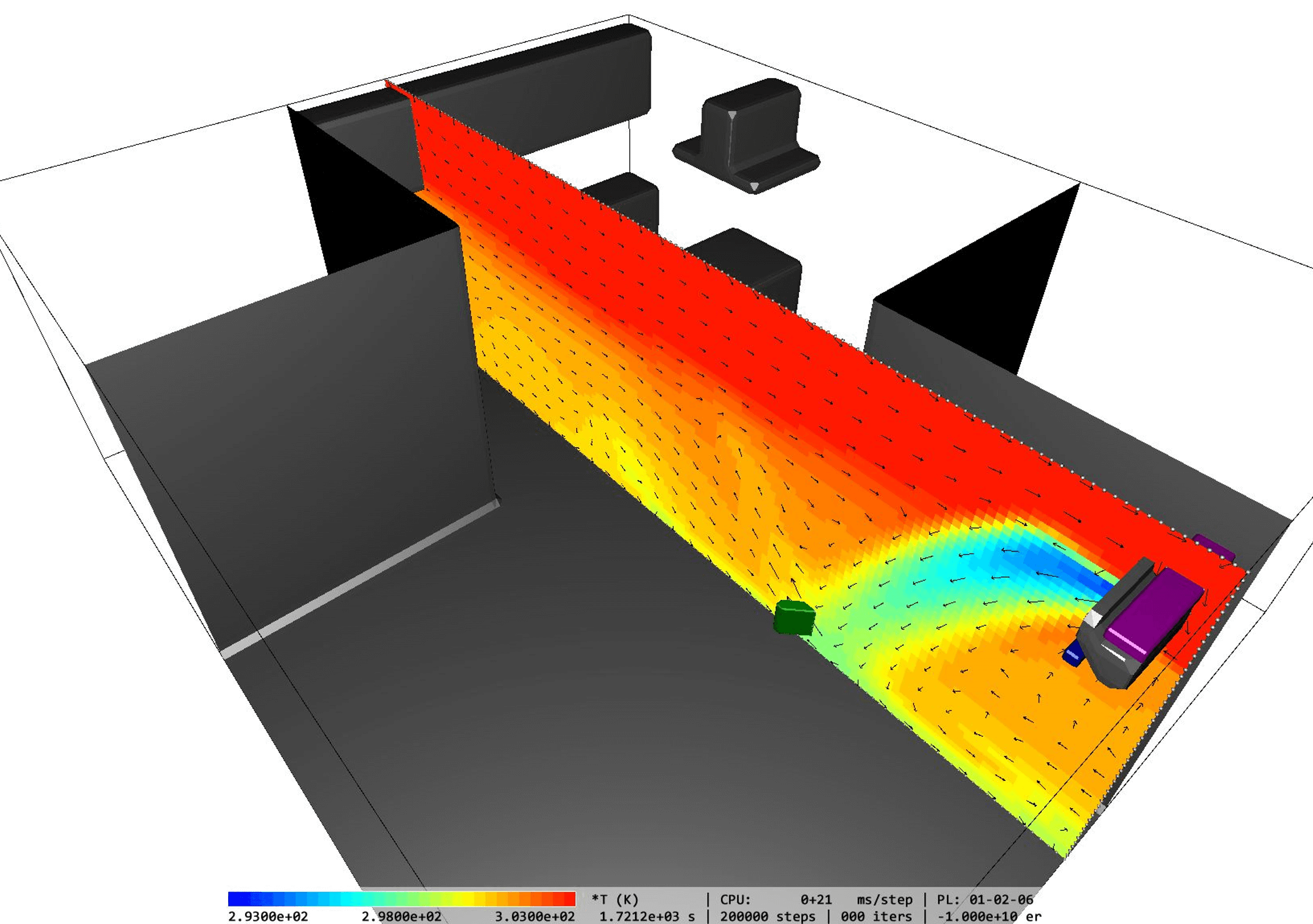
5. Simulation results
The temperature distribution visualization of simulation resutls for the refernece and combination cases are shown below. With a circulation fan, cooler air can be advected as far as the kitchen area.
You can perform a parametric study by considering different locations and directions of the circulation fan(s) for AC optimization.
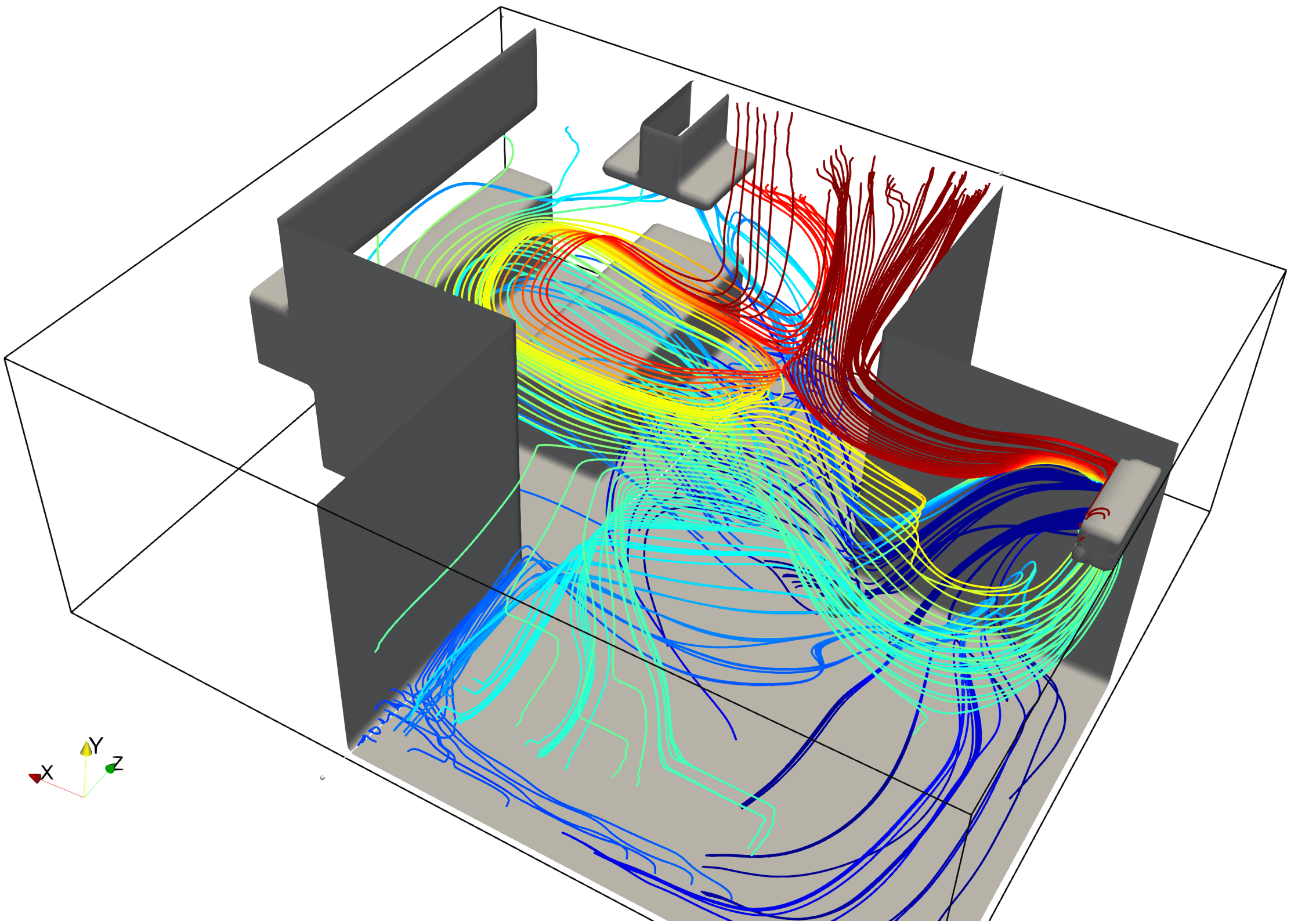
You can visualize the simulation result output data after the simulation by using the analysis mode in Flowsquare+. Also, these Flowsquare+ output data can also be visualized by any visualizing tool such as Paraview. Example visualization examples by using these two tools are shown below.