The Easiest Computational Fluid Dynamics Software
 JP
JP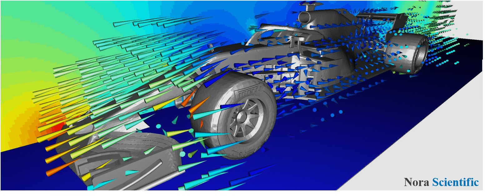
Wind Tunnel Test of F1 Model
The "preset boundary" is no longer available for 2021R2.0 or later. This example is modified so the boundary is now specified by a bitmap file.1. Introduction
Here on this page, a simlation case of a model F1 car is introduced, which could be used for benchmarking to understand Flowsquare+'s parallel computing performance and to explore computationally economical numerical conditions.
This simulation case is based on the one originally introduced on a user's website here (in Japanese), which were slightly modified for the present purposes.
The STL model we will simulate is freely available on 3Dmag.org, but if the link does not work, you can also obtain the same STL file from here as well.
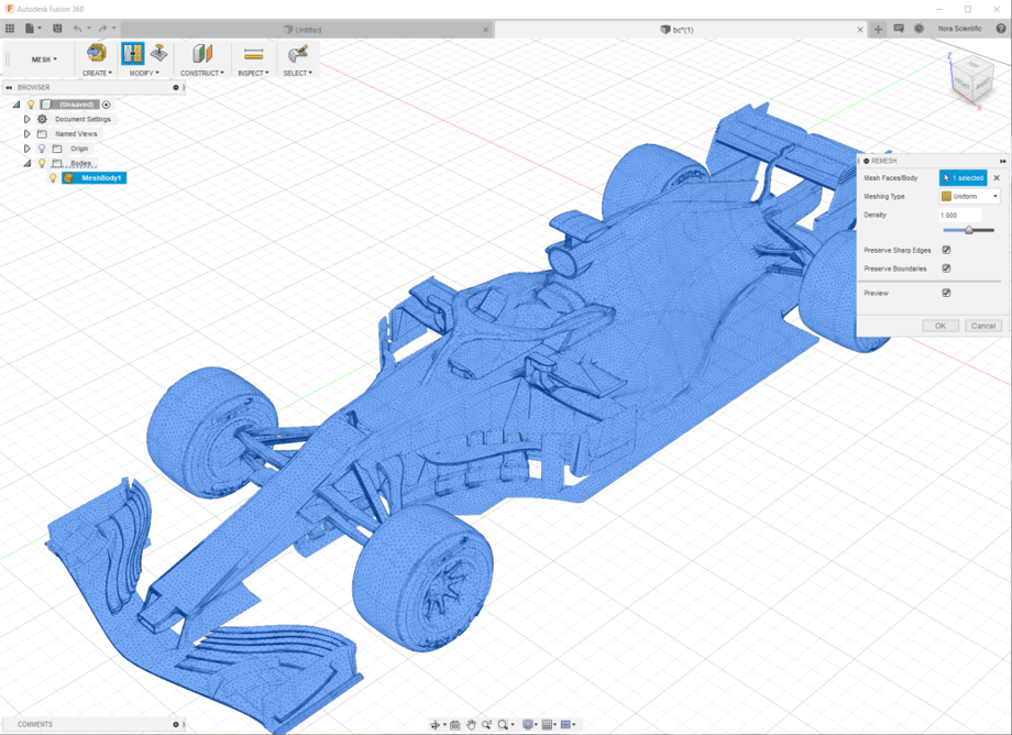
Before performing a simulation using this STL file, you may refer to "3D CAD Model and its Optimization", and remove unnecessary parts from the CAD model. An optimised STL file is included in the below input files, so you do not perform this optimization for the present simulation.
All the input files required for this simulation can be downloaded from below. Should you choose to download the zip file, you need to unzip the file, and store the unzipped files in somehwere under FSP directory or subdirectory.
Input files
A typical computational time of this case is approximately 1.2 hours per 1000 time steps with a typical Core i7 PC with the maximum parallelism setting (parallel in parameter setting)
2. Simulation domain
In this simulation, we will use a STL file and a bitmap image included above input files. Referring "Flowsquare+ for Beginners" page, please make a new project for the present simulation.
The bitmap image is shown below and only blue inflow boundary conditions are specified on the left and bottom of the domain.

Based on the bitmap image and the CAD model included in the above input files, the below simulation domain will be constructed. You may adjust position and angle of the CAD model (see "Boundary confirmation/CAD model loader" (in this example, the position and angle of the CAD model are already appropriately set). If you include STL-related parameters in the parameter set (as the above param.in does), the change of STL model position and rotation you perform in "Boundary confirmation/CAD model loader" is always saved in the parameters.
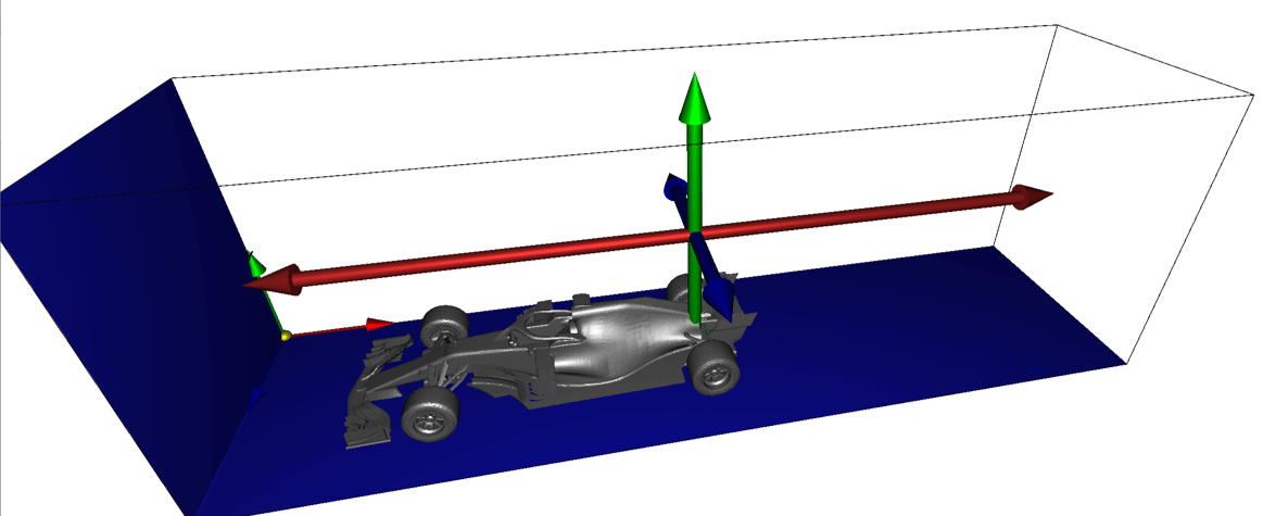
In the presen simulation, the domain length is approximately about only two times of the the object to reduce the computational cost. However, to avoid adverse effect of computational (open) boundaries, a domain length of 5-10 times of the object size is often considered. It would be a good idea, if large computational resource is available, to perform the similar simulations with different domain sizes, to check the effect of domain size on the solution.
3. Simulation parameters
This simulation requires a relatively huge computational time for most of PCs. The first few time steps are in particular slow. Thus, in the present simulation condition, loopmax value is changed from the default value of 1000 to 40. This yields a relatively large residual error in the beginning of the simulation, but it progressively decreases with the simulation time.
The blue boundary condition is used in the domain, so we need to specify velocity on the blue boundary. Comprehensive description of all parameters can be found here.
4. Simulation results
After performing the simulation, try various visualization tools using the Analysis mode. The top image on this page is one example of such a post visualisation.
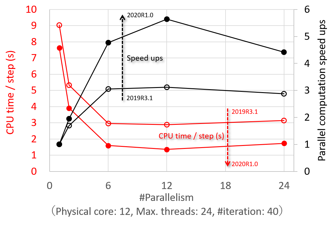
The below image shows computational time per time step at 100th time step of this simulation case for different parallelism (1, 2, 6, 12, 24 threads), comparing between two versions of Flowsquare+, 2019R3.1 and 2020R1.0.