The Easiest Computational Fluid Dynamics Software
 JP
JP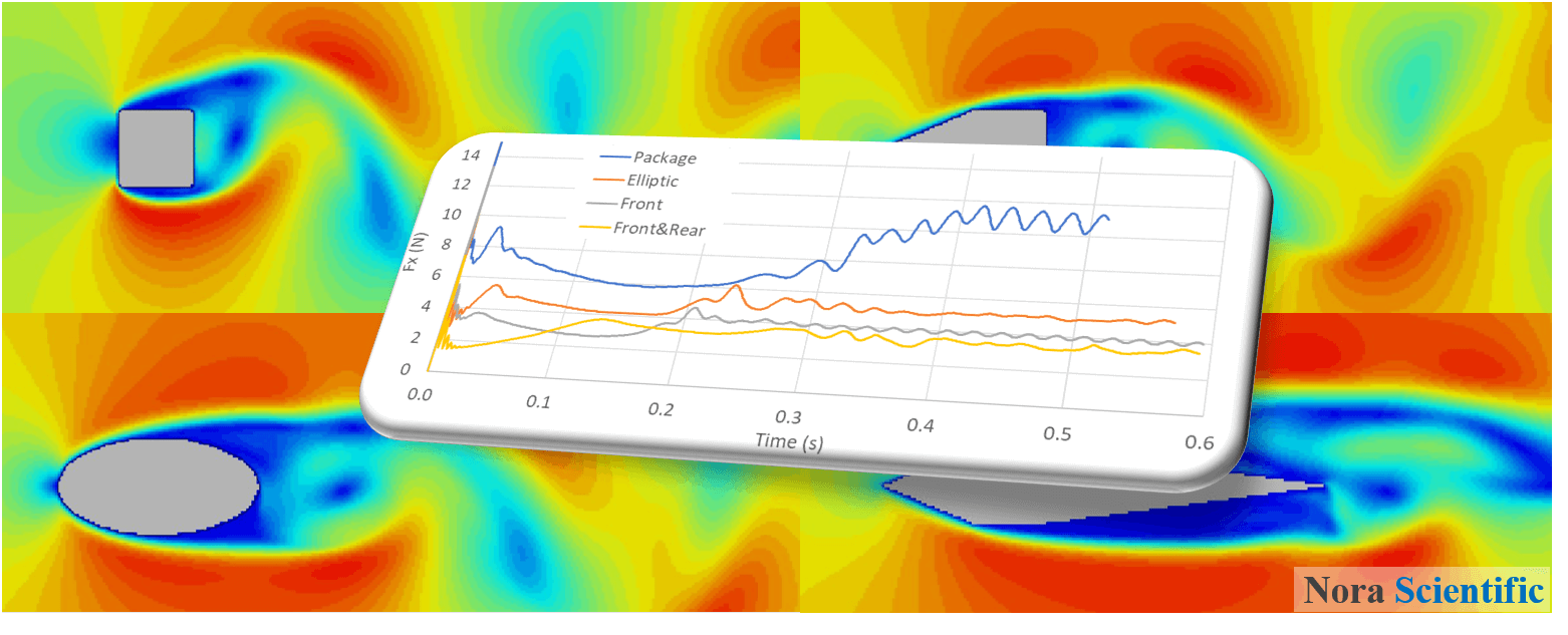
Minimum Drag Competition
1. Introduction
In this tutorial, the objective is to optimize the shape of aerodynamic attachments added to the "box" shown below in order to minimize the overall drag. The shape of the box itself must not be modified. You may also compete with other teams to see who can design the aerodynamic attachment that achieves the lowest drag.
Computaion and measurement of the hydrodynamic forces on an object using Flowsquare+ are explained here.
All the input files required for this simulation can be downloaded below.
"Box" case (without any aerodynamic part)
Example 1: Elliptic shape
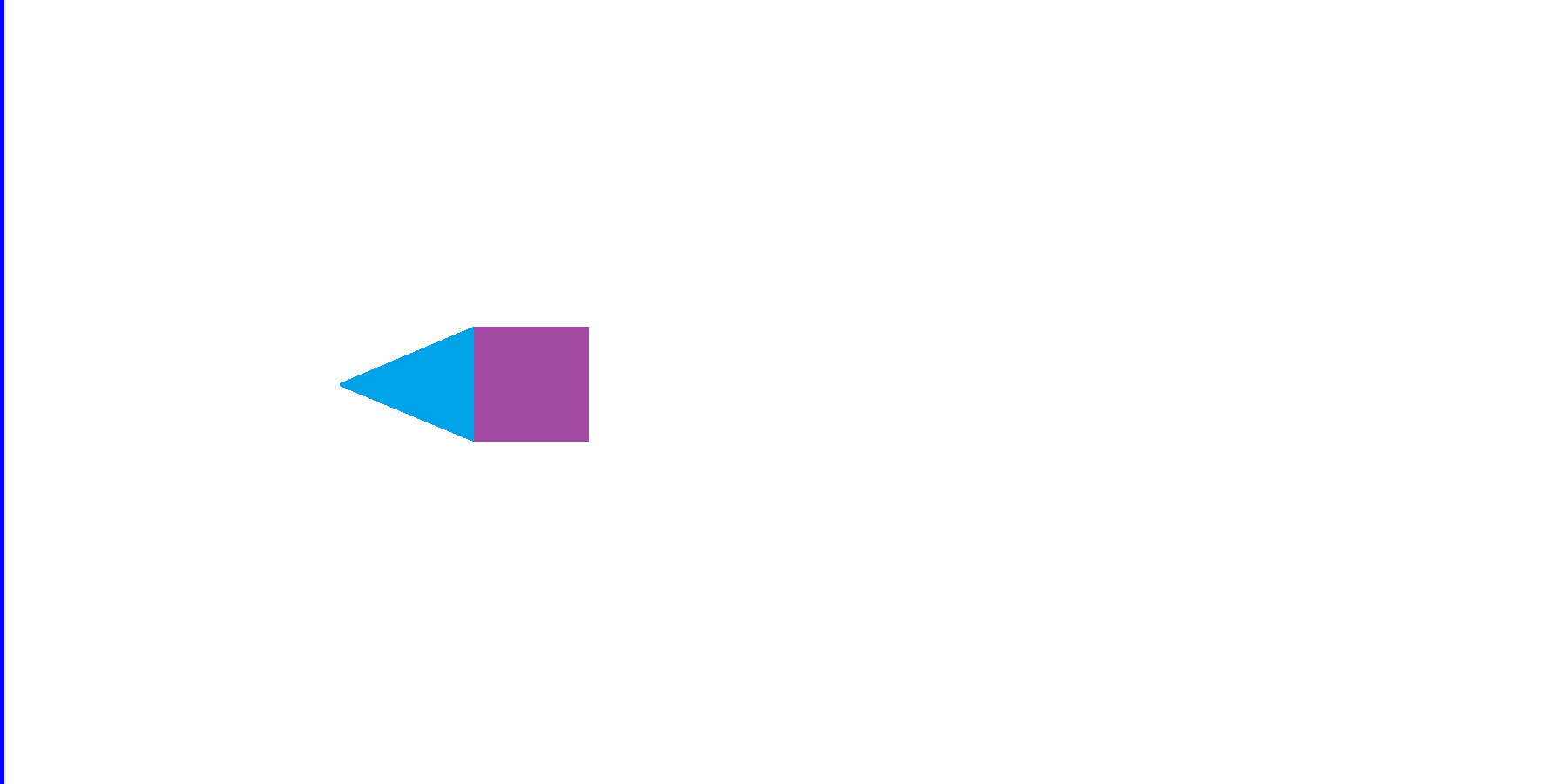
Example 2: Front wedge
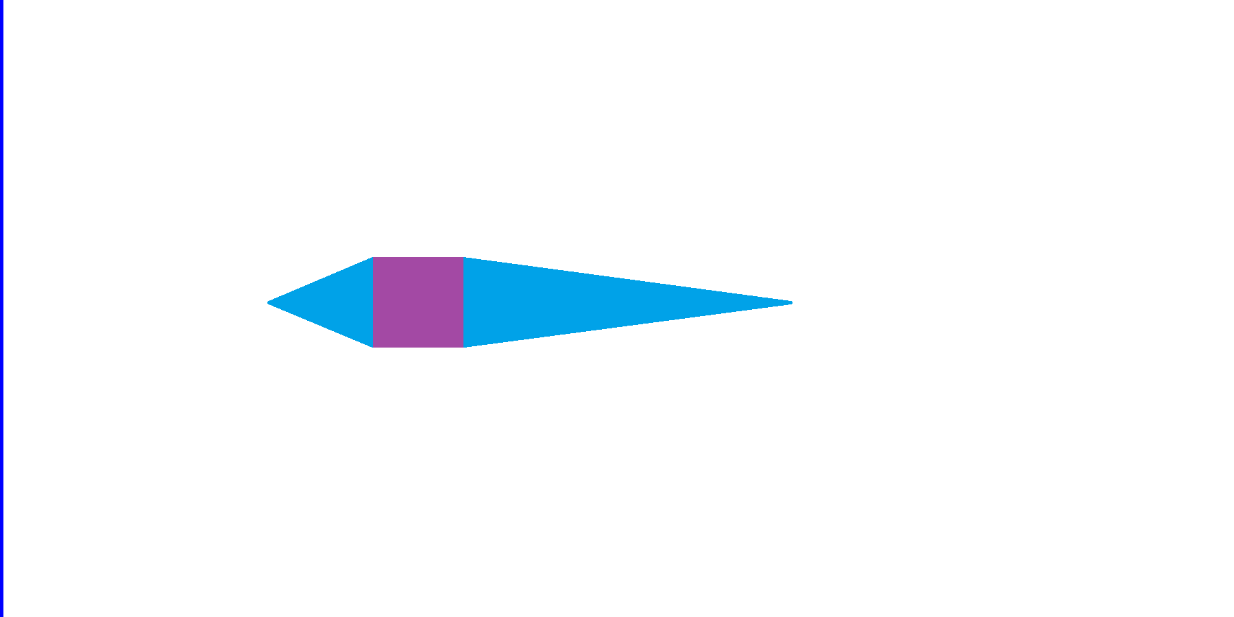
Example 3: Front & rear wedge
A typical computational time of this case is approximately 20 seconds per 1000 time steps with a typical Core i7 PC with parallel=3 setting (parallel in parameter setting).
2. Boundary condition (addition of aerodynamic parts)
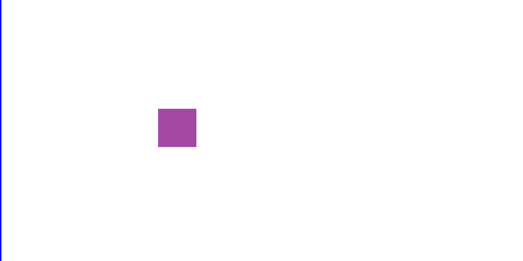
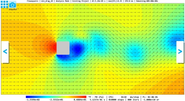
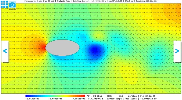
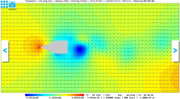
Following figures show the bitmap images for boundary condition specification (bcXY0.bmp). The mean flow direction is from the left to the right.
In this tutorial, we will minimize the hydrodynamic drag force by adding aerodynamic parts on the box denoted by the purple square on the bcXY0.bmp for the "box" case below. Three example designs are shown for a reference.


3. Simulation parameters
In the present simulations, drag reduction is achieved by modifying the shape of aerodynamic parts in bcXY0.bmp. For group competition for drag reduction, the same parameter setting may be used for different groups. Several important parameters are explained here. More thorough information about parameters can be found here.
- cmode
cmode is taken as 0 for the fluid simulation mode (constant density, constant temperature, single phase for gas and liquid flows).
- lx, ly
The domain lengths in X- and Y- directions are respectively 1.0m and 0.5m.
- nx、ny、nz
The number of mesh points needs be determined based on the required spatial resolution. Here, we will use (nx, ny, nz) = (400,2001), which yields the same mesh size for each direction.
- rhoW
Fluid density is taken as 1.2 kg/m^3, which corresponds to the air property at a standard condition.
- uinB
Inflow velocity at the blue inflow boundary is taken as 10m/s (36km/h).
4. Performing simulation
Using the input files doanloded from the above link and modify bcXY0.bmp for your own aerodynamic parts design. General steps to perform a simulation with Flowsquare+ are explained here. Also, computaion and measurement of the hydrodynamic forces on an object using Flowsquare+ are explained here.
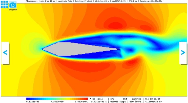
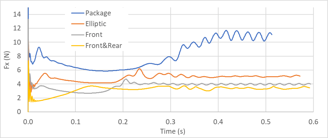
The instantaneous flow fields for the box alone (no aerodynamic part), and the cases with an elliptic part, front wedge and front and rear wedges are shown in below at 10,000-th step. Also, temporal variation of streamwise hydrodynamic forces acting on each of these objects are also shown.
Among the four cases (one without and three with aeroparts), the case with front and rear wedges achieves the smallest hydrodynamic drag force. How can we improve the design of the parts to lower the drag further?

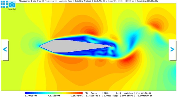
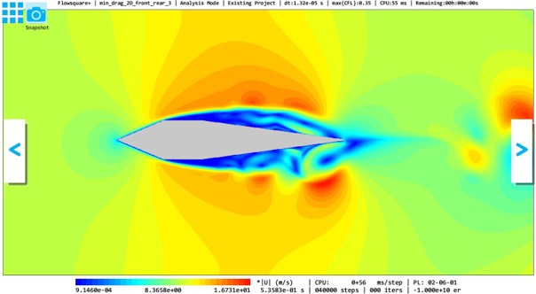
5. Spatial resolution dependency
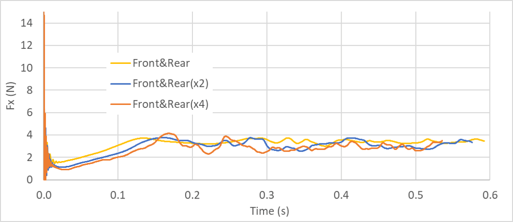
We will check the dependency of numerical results on the spatial resolution. Below figures show the flow field (velocity magnitude) and hydrodynamic force variation in time for the front & rear wedge cases with default spatial resolution (nx=400, ny=200), twice (nx=800, ny=400) and four times (nx=1600, ny=800) resoltion cases. The time step size decreases with the increase of resolution, so the simulations were continued until respectively latts=10,000、latts=20,000、latts=40,000.
Based on comparison of these three cases, with an increase of spatial resolution, velocity fluctuations with smaller length scales are captured, and time scale of unsteady motions seems to be slightly influenced. However, overall trend of measured hydrodynamic force does not seem to be unduly influenced qualitatively or quantitatively.