The Easiest Computational Fluid Dynamics Software
 JP
JP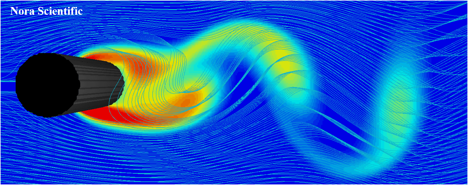
Karman Vortex in the Water
1. Introduction
Here we will introduce a simulation example of Karman vortex street in the water. Similar set ups are often used for student lab demostration in universities, and the simulation could be used for direct comparison with their measurements by varying the streamwise velocity and the diameter of the cylinder.
To change the cylinder diameter, it is easier to change the simulation domain dimensions, rather than modifying bcXY0.bmp. For example, by using half the sizes of original lx, ly, lz, essentially you can decrease the diamter (Reynolds number) by half.
All the input files required for this simulation can be downloaded from below.
Input files
A typical computational time of this case is approximately 2 minutes per 1000 time steps with a typical Core i7 PC with the maximum parallelism setting (parallel in parameter setting).
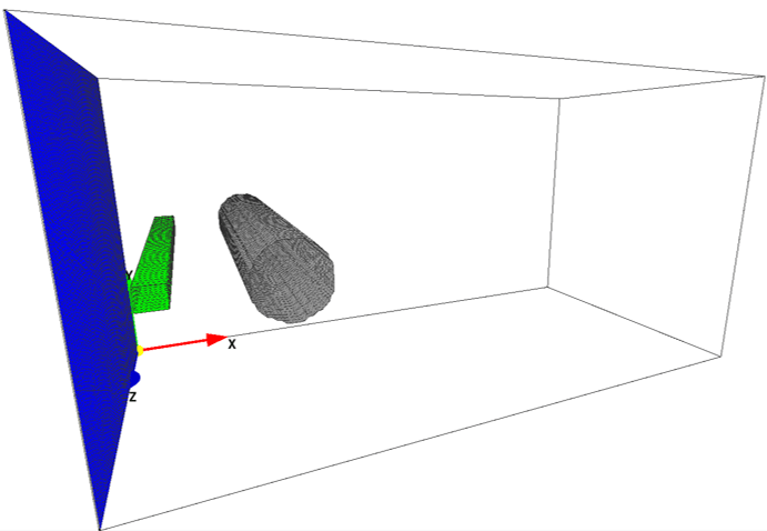
2. Domain configuration
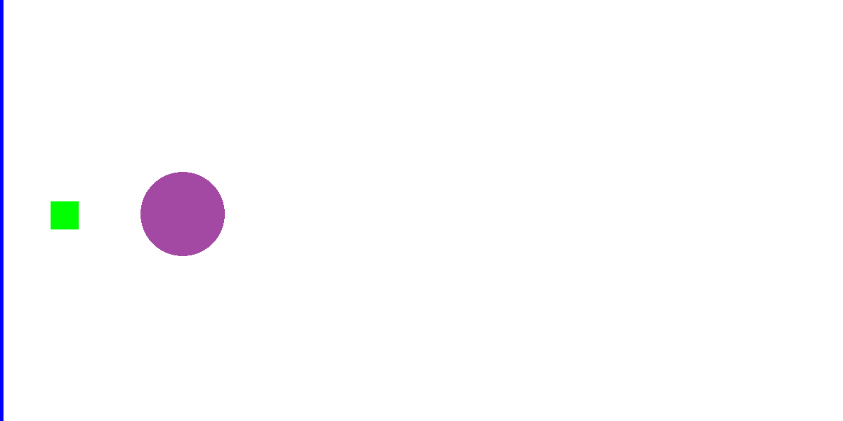
In the rectangular domain, there are an inflow boundary specificed by blue color, source of scalar (colored ink feed in the water) to visualize the flow field specified in green color in the downstream, and the solid wall (cylinder) to generate Karman vortex street specified by non-preset color or blank color.

3. Simulation parameters
Below explains several important aspects of the present simulation example. General description of parameters in Flowsquare+ are explained in here.
- lx, ly, lz
The domain dimensions are 0.6 x 0.3 x 0.3 (m^3). To modify the cylinder diameter, change the domain size.
- rhoW
Fluid density is taken as water's value of 1000 (kg/m^3).
- uinW, uinB
Initial velocity and blue inflow boundary velocity in x are specified as 1.0 (m/s).
- uinG, vinG, winG
The green boundary is used for scalar source (source of colored ink for visualization), and it should not influence the fluid velocity. Therefore, the inflow velocity (uinG, vinG, winG) is specified as "-" (hyphen).
- massfrG
The green boundary is the scalar source, so the mass fraction here is always fixed to 1.0. Mass fraction in other regions are zero by default.
- mu
The viscosity of water is 1.0E-3 (kg/m/s).
4. Simulation results
The simulation result is shown in movie below. The color shows the scalar mass fraction (colored ink feed in the water for visualization), and the small magenta box on the right hand side of the domain is the position of measurement probe.
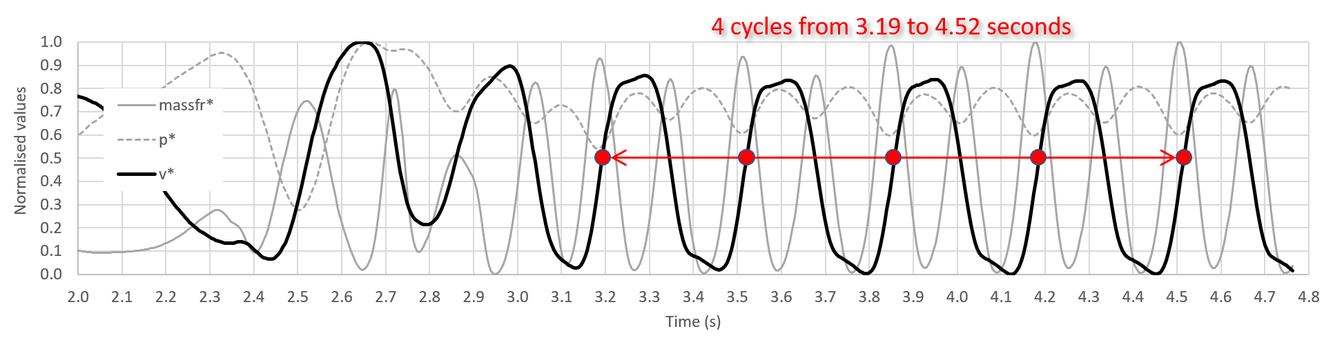
The measured data at this probe are shown below. Grey solid line is scalar concentration, grey dashed line is pressure, and black solid line is velocity component in y-direction. All the physical quantities are normalized by using their maximum and minimum value, bounded between 0 and 1. For example, the normalized value of a physical quantity \(q\) is calculated as \(q^*=(q-q_{min})/(q_{max}-q_{min})\).
In the present simulation setting, after reaching quasi-steady state, the cylinder diamter is 0.06 (m), inflow velocity is 1.0 (m/s), there are four cycles from 3.19 (s) until 4.52 (s), which yields oscillation frequency of 3.03 (1/s). The Strouhal number based on these values is 0.18, which is close to the empirical value of 0.2.