The Easiest Computational Fluid Dynamics Software
 JP
JP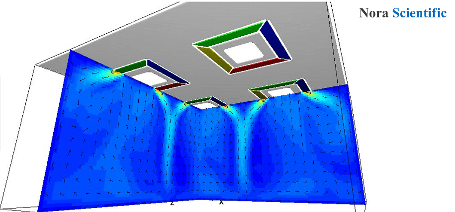
Simulation of 4-way cassette AC
1. Introduction
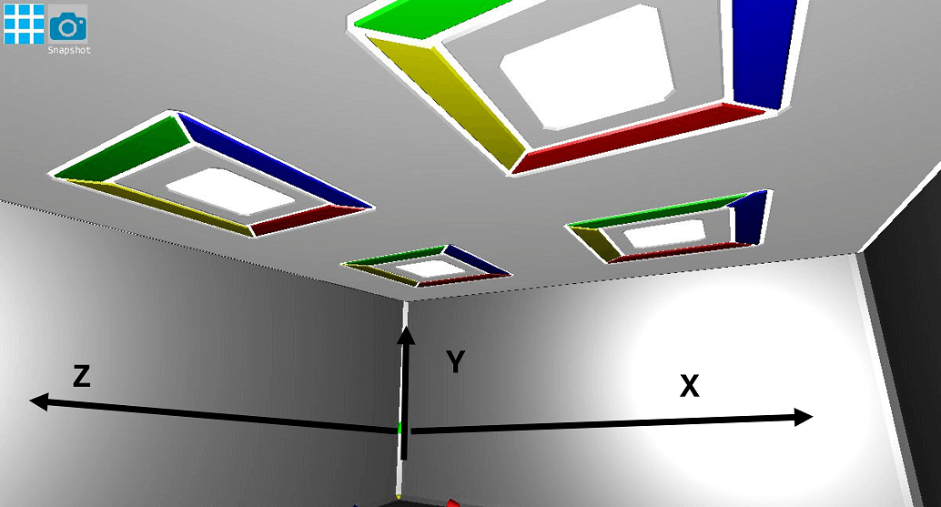
4-way cassette air conditioners are a type of air conditioning equipment installed mainly in ceilings. They have four-directional air outlets, which facilitate the uniform circulation of air in a room. They are often installed in offices and commercial facilities and look like the figure below.
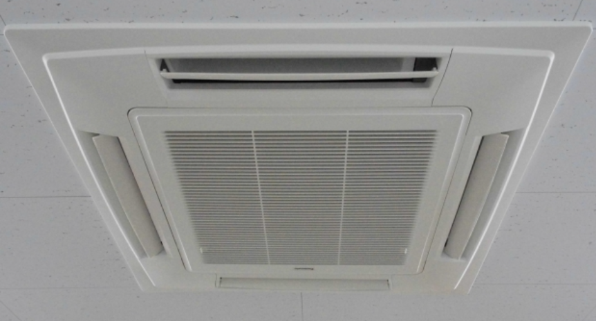
In such air conditioners, the slits on the four sides are air outlets, and air is often sucked in from the square in the middle.
This tutorial will show how to define such a relatively complex air outlet with boundary conditions. You can download all the input files necessary to run the simulations presented.
Input files
This simulation is performed on a typical Intel Core i7 laptop computer with a parallel level of "parallel = 3" (see parameter setting) at a computational cost of about 1 minute per 1000 steps.
2. 3D model construction
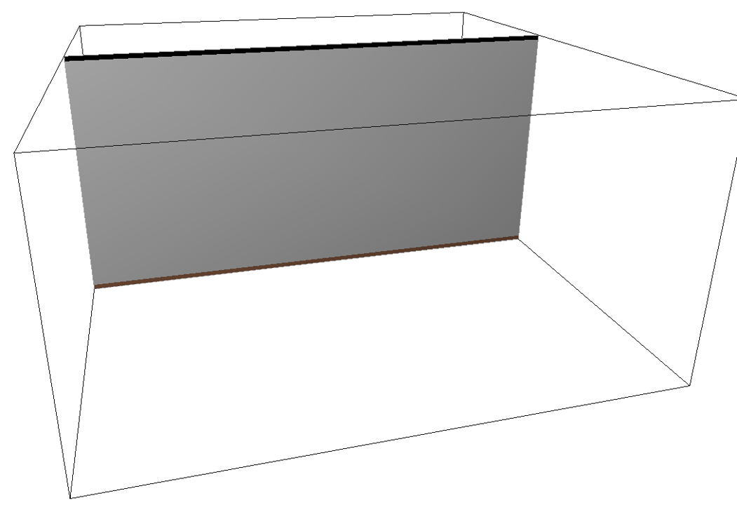
Please refer to this page for the basic construction rules for creating the 3D model. The first step is to create bitmap images for each boundary element.
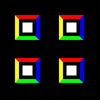
In this simulation, bitmap images for boundary conditions are created using the following preset colors to represent a 4-way air outlet. The inlet is assumed to be a natural outflow (of course, forced outflow can be specified).
Preset colors- ■ Positive x-directional air vents
- ■ Negative x-directional air vents
- ■ Positive z-directional air vents
- ■ Negative z-directional air vents
- ■ Ceiling
- ■ Floor
- ■ Wall
It is recommended that these boundary condition colors be determined gradually while creating and checking each element part.
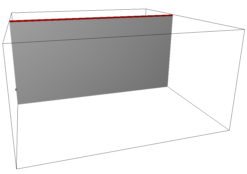
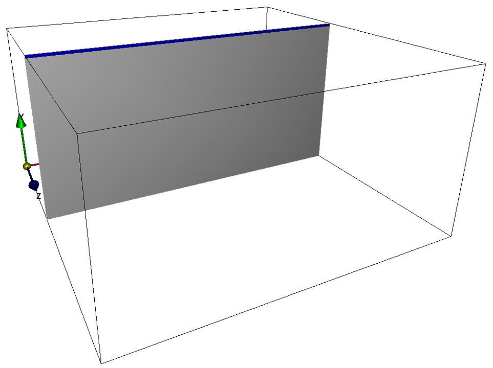
The figure below shows the orientation of the bitmap image for boundary conditions within the simulation area.
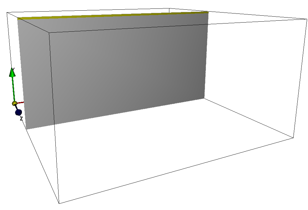
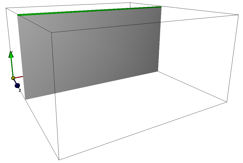
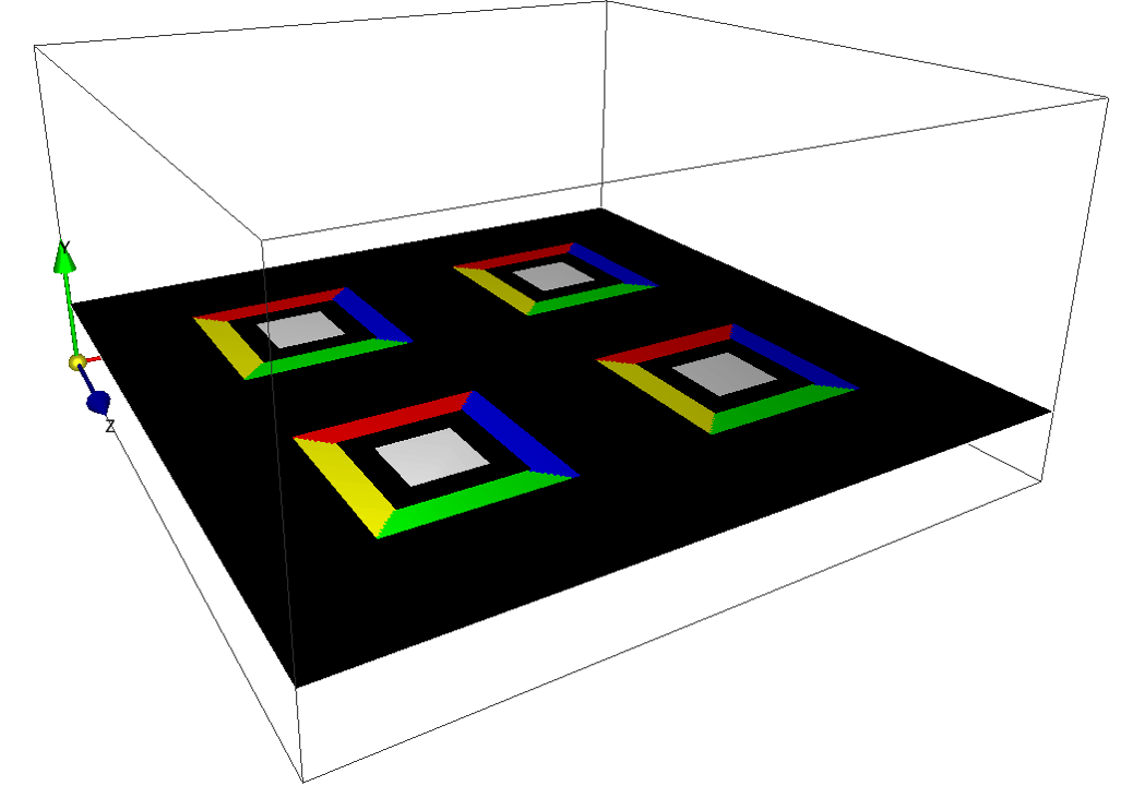

Based on these bitmap images of boundary conditions, an office space with 4-way cassette air conditioners is constructed as shown below. The boundary conditions are such that blue, red, yellow, and green slits blow out in all directions. The square area in the center of these air outlets will be the intake (natural outflow this time).
3. Input parameters
The following describes parameters of particular importance in this simulation. For a description of general calculation parameters, please click here.
- cmode
0: fluid simulation mode (no density or temperature fluctuations) is selected. To simulate cooling and heating, select the thermo-fluid mode with cmode=1 and add temperature conditions seperately. - lx, ly, lz
The simulation domain sizes in x-, y-, and z-directions are 5.0 m, 2.5 m, and 5.0 m, respectively. - nx, ny, nz
The number of mesh points in the x, y, and z directions is determined by considering the required spatial resolution and computational resources. In this tutorial, (nx, ny, nz) = (100, 50, 100). - uinB, vinB, winB
From the blue boundary, positive x-directional and downward inflow (uinB, vinB, winB) = (2.0, -1.0, 0.0) m/s - uinY, vinY, winY
From the yellow boundary, negative x-directional and downward inflow (uinY, vinY, winY) = (-2.0, -1.0, 0.0) m/s - uinG, vinG, winG
From the green boundary, positive z-directional and downward inflow (uinG, vinG, winG) = (0.0, -1.0, 2.0) m/s - uinB, vinB, winB
From the red boundary, negative z-directional and downward inflow (uinR, vinR, winR) = (0.0, -1.0, -2.0) m/s - mu
The viscosity coefficient of air is specified as 2.0E-5 (kg/m/s).
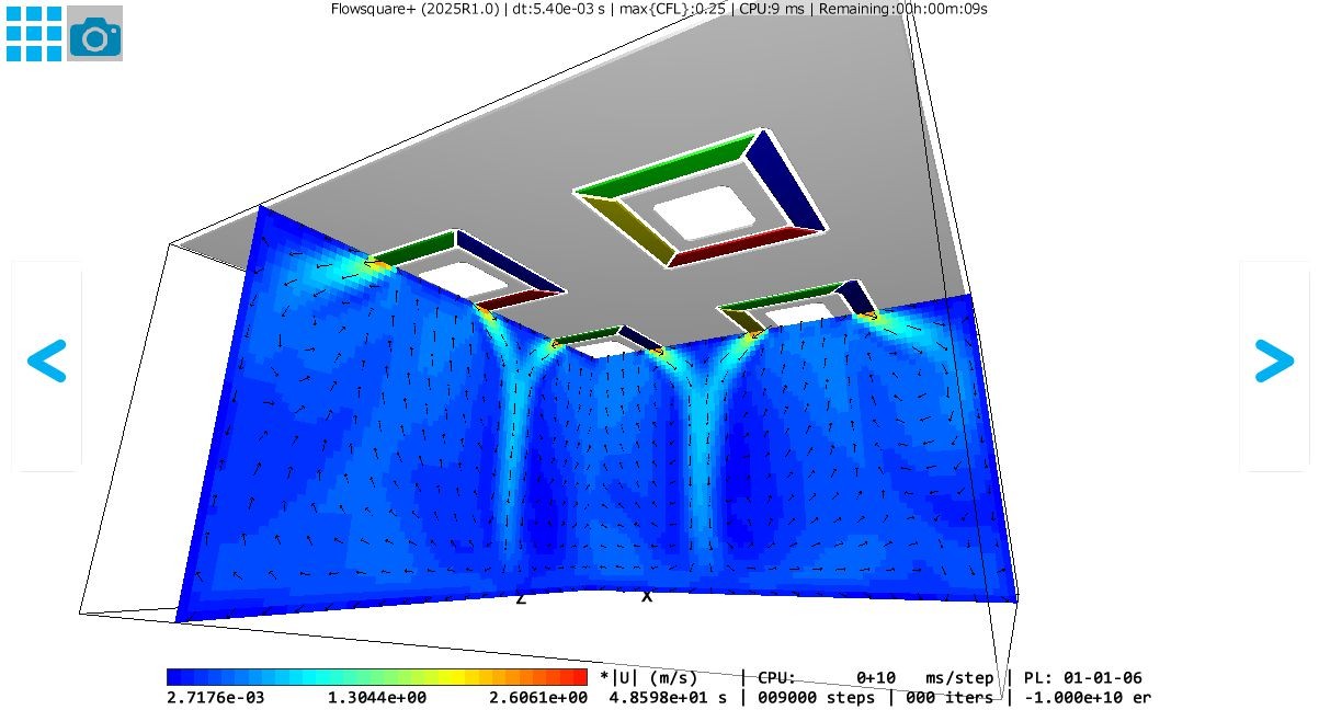
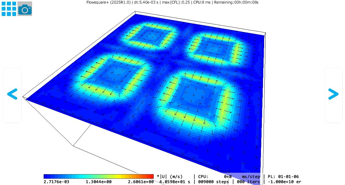
4. Simulation results
The results of running Flowsquare+ with this simulation input file are as follows.