The Easiest Computational Fluid Dynamics Software
 JP
JP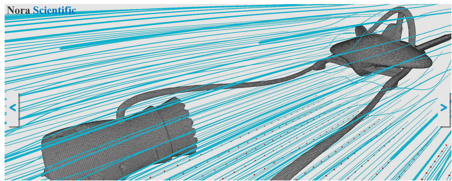
Flow Analysis around a Pod Racer
The "preset boundary" is no longer available for 2021R2.0 or later. This example is modified so the boundary is now specified by a bitmap file.1. Introduction
In this example, we will learn how to specify a simulation domain with a CAD model and a paint image.
The model we will simulate is a "pod racer" appearing in Star Wars films. The original pod racer cad file is freely available on GRABCAD, but if the link does not work, you can also obtain the same STL file from here as well.
Before performing a simulation using this STL file, you may refer to "3D CAD Model and its Optimization", and remove unnecessary parts from the CAD model. An optimised STL file is included in the below input files, so you do not perform this optimization for the present simulation.
All the input files required for this simulation can be downloaded from below. Should you choose to download the zip file, you need to unzip the file, and store the unzipped files in somehwere under FSP directory or subdirectory.
Input files
A typical computational time of this case is approximately 5 minutes per 1000 time steps with a typical Core i7 PC with the maximum parallelism setting (parallel in parameter setting).
Referring "Flowsquare+ for Beginners" page, please make a new project for the preent pod racer simulation.
2. Simulation domain
In this simulation, we will use a STL file included above input files, and a bitmap image. The bitmap image is shown below and only blue inflow boundary conditions are specified on the left and bottom of the domain.

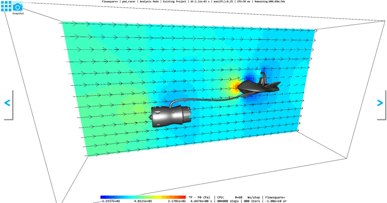
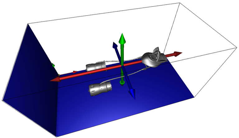
Based on the above bitmap image and the CAD model included in the above input files, the below simulation domain will be constructed. You may adjust position and angle of the CAD model (see "Boundary confirmation/CAD model loader" (in this example, the position and angle of the CAD model are already appropriately set). If you include STL-related parameters in the parameter set (as the above param.in does), the change of STL model position and rotation is always saved in the parameters.
3. Simulation parameters
The blue boundary condition is used, so we need to specify velocity on the blue boundary. Detailed information about parameters can be found here.
- cmode
cmode is taken as 0 for the fluid simulation mode (constant density, constant temperature, single phase for gas and liquid flows).
- uinB
Inflow velocity in X-direction on the blue inflow boundary is taken as 20.0 m/s.
- unitSTL, xOffstSTL, yOffstSTL, zOffstSTL, xRotSTL, yRotSTL, zRotSTL
Length unit, position and rotation angle of the CAD model can also be specified graphically in the "Boundary confirmation/CAD model loader" (in this example, the position and angle of the CAD model are already appropriately set).
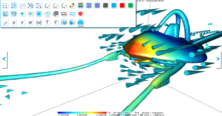
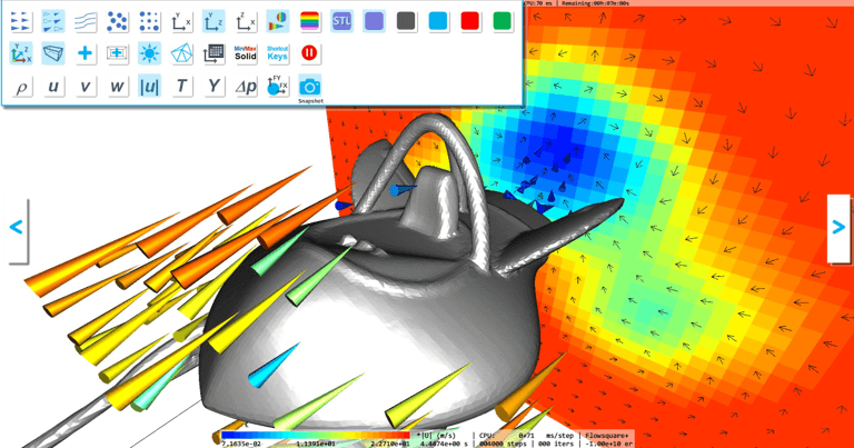
4. Simulation results
After performing the simulation, try various visualization tools using the Analysis mode. Of course, these visualization tools can be used during the simulation too.