The Easiest Computational Fluid Dynamics Software
 JP
JP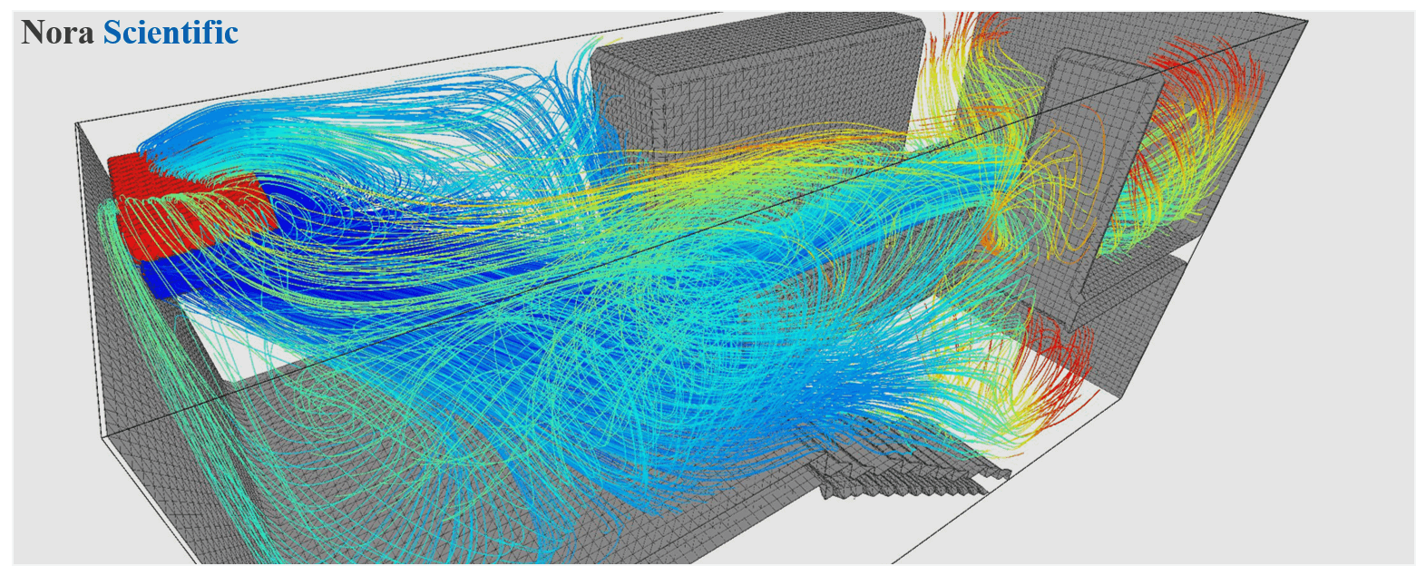
Room AC Cooling Simulation
1. Introduction
Here, we will learn 3D modeling, input files and some visualization tips for intuitive understanding through a simulation of AC cooling in a room. Similar simulations could be used for parametric study for optimization of AC equipment arrangement.
All the required input files for this test case can be downloaded below.
Input files
A typical computational time of this case is approximately 5 minutes per 1000 time steps with a typical Core i7 PC with the maximum parallelism setting (parallel = 4 in parameter setting).
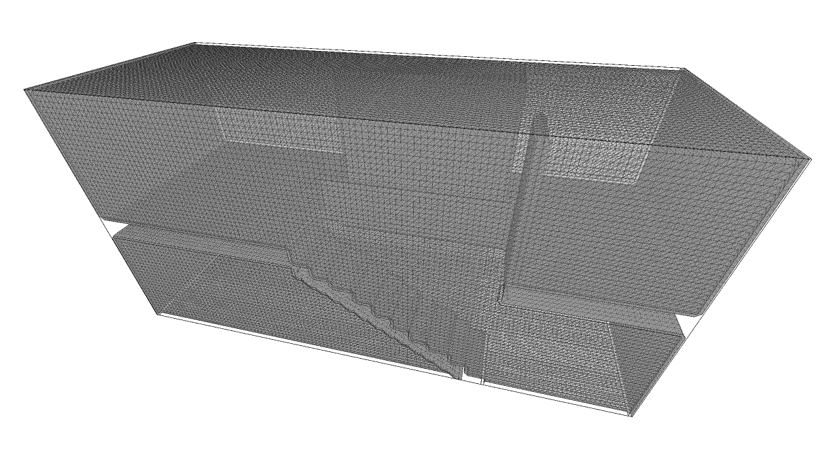
2. 3D model construction
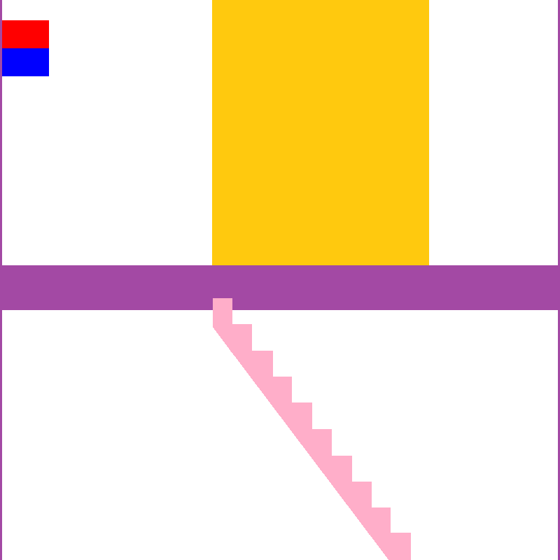
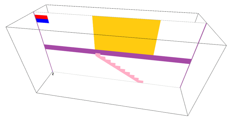
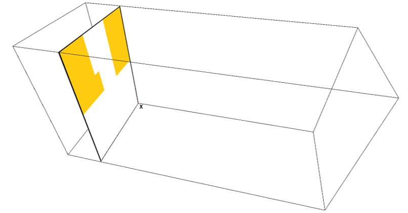
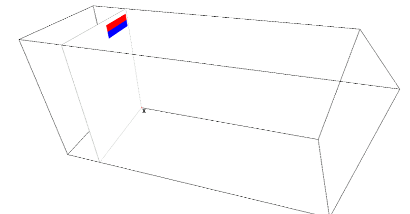
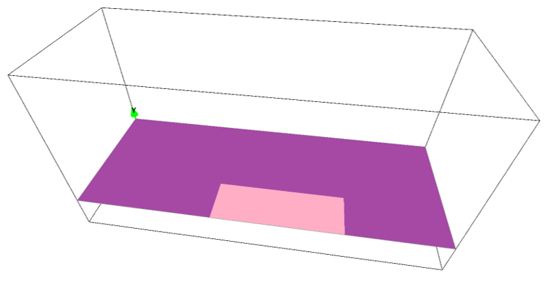
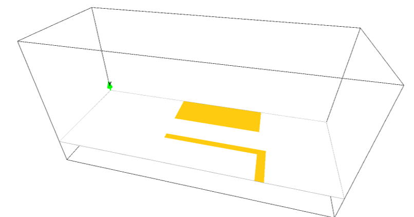
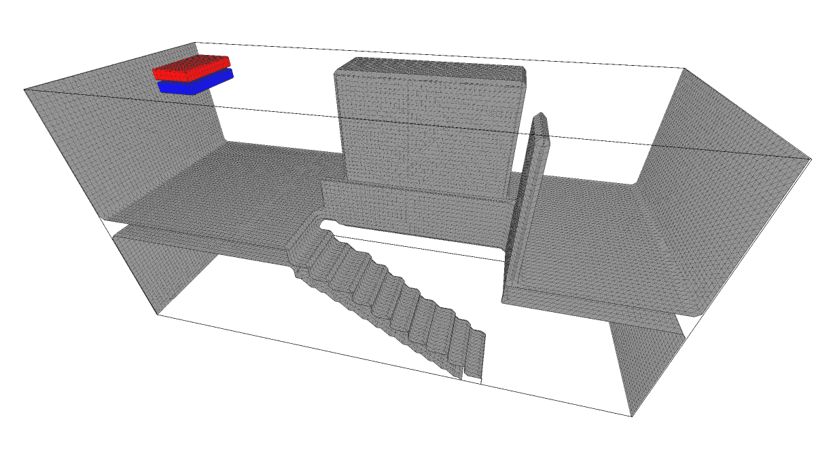
General rules of constructing 3D boundary conditions using paint images are explained in here. In the present simulation, following five paint images are used to construct the model of a 2-story apartment. The six colors used in the paint images and parts these colors specify are:
- Non-preset color, purple: 1st floor ceiling and 2nd floor floor, and walls on right and left hand sides in X-directions.
- Non-preset color, pink: Stairs.
- Non-preset color, yellow: Dividing walls on the 2nd floor.
- Preset color, red: Air intake of the AC (room-temperature air flows into AC from here).
- Preset color, blue: Air outlet of the AC (cooled air comes out from here).
- Preset color, black: Foreground and background walls, and 1st floor floor and 2nd floor ceiling.
The paint image pixel sizes can be irrelevant to actual physical domain dimensions. The model dimensions are specified by the parameters, lx, ly and lz. However, it is a good habit to use more or less similar aspect ratio between images and domain dimensions.
3. Numerical parameters
Several important parameters are explained here. More thorough information about parameters can be found here.
- cmode
cmode is taken as 1 for the 1:Thermo fluid simulation mode (varying temperature ideal-gas flows).
- lx
The domain length in X-direction is 8m.
- ly
The domain length in Y-direction is 4m.
- lz
The domain length in Z-direction is 3m.
- nx、ny、nz
The number of mesh points needs be determined based on the required spatial resolution. Here, we will use (nx, ny, nz) = (120, 60, 45), to yield equal mesh density for all directions.
- tempW
Initial air temperature in the domain is set to be 310K (approximately 37 degrees C). - uinW, vinW, winW
Initial velocity in the domain is 0.0m/s, which are default values of these parameters. Therefore they do not need to be specified in the parameter file. - uinB、vinB、winB
The outflow velocity from the AC are set to be uinB = 2.0m/s, vinB = -2.0m/s (minus sign means direction towards down), and winB = 1.0m/s. The magnitude of the outflow velocity is 3.0m/s. - uinR、vinR、winR
The intake flow velocity to the AC is set to be uinR = 0.0m/s, vinR = -3.0m/s (again, minus sign means direction towards down), winR = 0.0m/s. The magnitude of this velocity is 3.0m/s, which is the same as magnitude of outflow velocity, to ensure the conservation of mass. - tempB
The temperature of the outflowing fluid from the AC is set to be 300K (27 degrees C). - tempR
The temperature of the intake air to the AC is set as adiabatic (tempR=0.0). - tempWallK, tempWall
The temperature conditions for walls specified by the preset black color and non-preset colors are adiabatic (0). - gfy
To include the buoyancy (warmer air goes up, cooler air goes down), Y-direction external force is also specified as -9.8 m/s^2 (minus sign means direction towards down).
4. Performing simulations, post-analysis
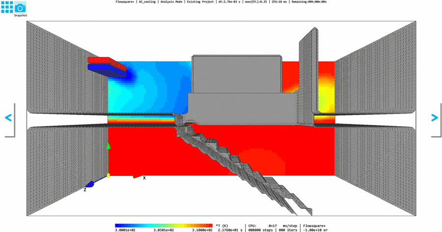
After performing the simulation, you can visualize the simulated and saved instantaneous field in the analysis mode. This allows you to closely examine the simulated flow field. The below gif image shows typical simulation result of the present case.
Also, you can place measuring probes in the simulation domain (room) to obtain temporal evolution of various quantities at fixed locations.